MatSQ has modularized each function, making it easy to add and modify functions.
The simulation module, Quantum Espresso (QE), is intended to perform electronic structure calculations using Quantum Espresso, an open-source DFT calculation software package. MatSQ provides an intuitive graphical interface (GUI) that makes it easy to perform DFT calculations with just a few clicks without studying complex codes. Most calculations can achieve good results by simply changing major keywords, such as cutoff energy and k-point, in the basic preset parameters. Moreover, MatSQ provides the manual mode for modifying scripts directly for experienced users.
For more information about Quantum Espresso, go to the appendix or www.quantum-espresso.org .
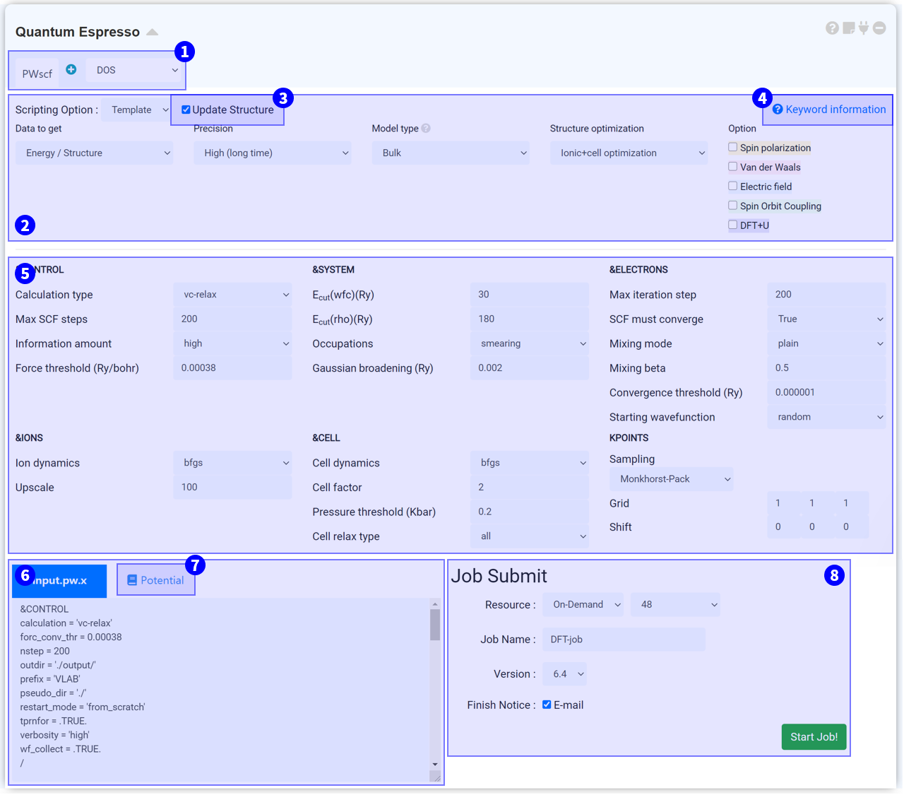
Solvers are major calculation programs used in Quantum Espresso package. Each Solver has a specific role, and can be divided into PWscf (pw.x) for scf calculations and post-processing solvers. PWscf is the most basic tab for obtaining all data. It performs self-consistent calculations on electronic structural properties using the Plane-Wave (PW) basis set and pseudopotentials (PP, psp). SCF calculations must be performed to obtain DFT simulation data, so the QE modules are configured around PWscf. Performing post-processing calculations is simple.
On QE modules that have already finished PWscf calculations, you can add a post-processing solver, and press the Start Job! to obtain additional post-processing data.
Information about input script settings for each solver can be found in the Appendix or ④ Keyword Information.
Press the Scripting Option to view Template, General, and Manual options. Template is a good option for those who are not familiar with the keyword settings in Quantum Espresso. In Template, you answer to several questions to set the input script.
Quantum Espresso modules get structural information from the connected Structure Builder. When the Structure Builder changes, the changed structural information is also updated on the QE module. If you do not want to update the structural information of the QE module anymore, untick this checkbox.
Each solver has a different set of input parameters. For more information, click on ? Keyword information to connect to the following URL:
MatSQ makes it easy to perform DFT calculations with just a few clicks. Input parameters, which are set by default in the Quantum Espresso module, are roughly set with typical values. Most calculations can achieve good results simply by changing major keywords such as cutoff energy and k-point. However, the values should be carefully considered and selected based on an understanding of each input parameter to perform reliable DFT simulations for advanced use such as research and papers.
For more information, refer to the appendix or ④ Keyword Information.
An input script is created when the QE module is connected to Structure Builder, and input parameters are set. The input script is a text that has structure information and keyword setting information sent to the cloud server. Therefore, it is recommended that you always ensure the values you set are correctly applied. When you change the option to Manual in ② Scripting Option, the ⑤ Input Parameters section is omitted, and only the Input Script window remains to allow you to modify the script manually. When you modify text in the Input Script window, the mode automatically changes to Manual.
Pseudopotentials are used to determine the behavior of the corresponding elements when using Quantum Espresso to perform DFT calculations. Click on the magnifying glass icon on the Pseudopotential tab to view the list of available pseudopotentials. Please refer to the Quantum Espresso Official Documentation for further information on pseudopotential.
After finishing the setting, submit the job to cloud server by referring to the Job submit section.
If you connect a new QE module to the QE module that has finished the calculation, you can proceed with further calculations from the last point with “restart.” Especially, you can restart the calculation that has been interrupted by the user request. But please note that the errored calculation cannot be restarted. It is recommended that you apply this function in the following cases:
Cases 3 and 4 are to restart calculations by rearranging the k-point used in the finished PWscf (pw.x) calculation. In Case 4, change the calculation type to nscf and set the k-point grid to more dense. As the nscf calculation means a non-self-consistent field calculation and only changes the k-point sampling density, it saves computing resources when compared with the dense k-point setting in scf (relax) calculations. In Case 5, change the calculation type to bands, and set the k-point as desired. It is recommended that you select crystal (_b) as the k-point option to sampling the high-symmetric point to get a good band structure. However, restarting a job calculated with the GAMMA option with the automatic option is not supported.
For more information about Quantum Espresso, go to the appendix or www.quantum-espresso.org .
Solvers are major calculation programs used in Quantum Espresso package. Each Solver has a specific role, and can be divided into PWscf (pw.x) for scf calculations and post-processing solvers. PWscf is the most basic tab for obtaining all data. It performs self-consistent calculations on electronic structural properties using the Plane-Wave (PW) basis set and pseudopotentials (PP, psp). SCF calculations must be performed to obtain DFT simulation data, so the QE modules are configured around PWscf. Performing post-processing calculations is simple.
- Add a QE module, and in ① Solver region, click on a solver (DOS, Charge density, ...) that is suitable for obtaining the desired data.
- Then press the + button to add a new solver tab next to the PWscf calculation. Add as many post-processing solvers as you want.
- Press the Start Job! button to run all calculations that have been added upon QE module.
On QE modules that have already finished PWscf calculations, you can add a post-processing solver, and press the Start Job! to obtain additional post-processing data.
Information about input script settings for each solver can be found in the Appendix or ④ Keyword Information.
Press the Scripting Option to view Template, General, and Manual options. Template is a good option for those who are not familiar with the keyword settings in Quantum Espresso. In Template, you answer to several questions to set the input script.
- Target property : Select what data you want to get. A Solver is added according to match the answer.
- Precision : It sets the precision level of calculations.
- Model type : This question is added when you select “High precision” to the previous question. Select the classification of the Simulation model. Determine the k-point format.
- Structure optimization : This is the question that determines the calculation type. If you select “Fully optimized,” it sets the calculation type to “scf” and does not change the initial structure during the calculation process. If you select “Need optimization / Need ionic+cell optimization,” it slightly changes the atomic position / atomic position + cell size and locates the “global minimum” in the potential surface to perform structure/cell optimization.
- Option : It decides which calibration to add. Spin polarization and Van der Waals correction are currently available.
Quantum Espresso modules get structural information from the connected Structure Builder. When the Structure Builder changes, the changed structural information is also updated on the QE module. If you do not want to update the structural information of the QE module anymore, untick this checkbox.
Each solver has a different set of input parameters. For more information, click on ? Keyword information to connect to the following URL:
- pw.x: https://www.quantum-espresso.org/Doc/INPUT_PW.html
- projwfc.x: https://www.quantum-espresso.org/Doc/INPUT_PROJWFC.html
- pp.x: https://www.quantum-espresso.org/Doc/INPUT_PP.html
- bands.x: https://www.quantum-espresso.org/Doc/INPUT_BANDS.html
MatSQ makes it easy to perform DFT calculations with just a few clicks. Input parameters, which are set by default in the Quantum Espresso module, are roughly set with typical values. Most calculations can achieve good results simply by changing major keywords such as cutoff energy and k-point. However, the values should be carefully considered and selected based on an understanding of each input parameter to perform reliable DFT simulations for advanced use such as research and papers.
For more information, refer to the appendix or ④ Keyword Information.
An input script is created when the QE module is connected to Structure Builder, and input parameters are set. The input script is a text that has structure information and keyword setting information sent to the cloud server. Therefore, it is recommended that you always ensure the values you set are correctly applied. When you change the option to Manual in ② Scripting Option, the ⑤ Input Parameters section is omitted, and only the Input Script window remains to allow you to modify the script manually. When you modify text in the Input Script window, the mode automatically changes to Manual.
Pseudopotentials are used to determine the behavior of the corresponding elements when using Quantum Espresso to perform DFT calculations. Click on the magnifying glass icon on the Pseudopotential tab to view the list of available pseudopotentials. Please refer to the Quantum Espresso Official Documentation for further information on pseudopotential.
After finishing the setting, submit the job to cloud server by referring to the Job submit section.
If you connect a new QE module to the QE module that has finished the calculation, you can proceed with further calculations from the last point with “restart.” Especially, you can restart the calculation that has been interrupted by the user request. But please note that the errored calculation cannot be restarted. It is recommended that you apply this function in the following cases:
- When the “This job is not converged” message is displayed;
- When the “This job is normally finished” message appears but the “max scf step” set by “scf step” is reached (in case of (vc-)relax);
- When you want to increase the k-point for DOS calculations; or
- When you want to set the k-point to the high-symmetric point path for band structure calculations.
Cases 3 and 4 are to restart calculations by rearranging the k-point used in the finished PWscf (pw.x) calculation. In Case 4, change the calculation type to nscf and set the k-point grid to more dense. As the nscf calculation means a non-self-consistent field calculation and only changes the k-point sampling density, it saves computing resources when compared with the dense k-point setting in scf (relax) calculations. In Case 5, change the calculation type to bands, and set the k-point as desired. It is recommended that you select crystal (_b) as the k-point option to sampling the high-symmetric point to get a good band structure. However, restarting a job calculated with the GAMMA option with the automatic option is not supported.
The 'Reaction Path (NEB)' module is for calculating Nudged Elastic Band (NEB) calculation by the neb.x solver provided by Quantum Espresso.
In order to perform NEB calculations, you must add the initial, final images (if necessary, up to the intermediate image) to the structure list in the 'Structure Builder' connected to the 'Reaction Path (NEB)' module. For a better results, all the images should be optimized (relaxed).
See the Quantum Espresso Input description (neb.x) for a detailed explanation of the NEB input script settings.
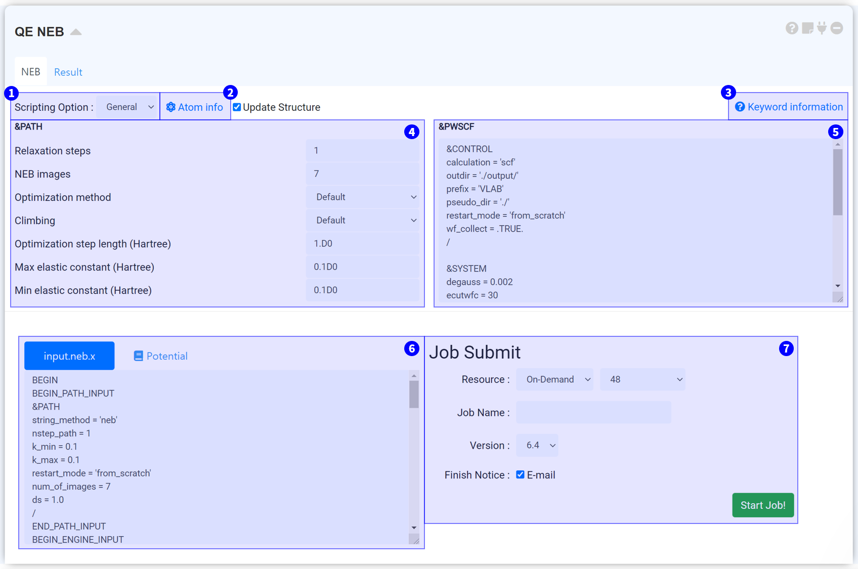
You can select General and Manual mode in the Reaction Path (NEB) module.
It is a tool for fixing some atoms during the NEB path. The tab number means the order of the structure list in the connected structure builder. If you select atoms you want, the atoms will consider fixed during NEB calculation.
This is a link to see a list of all keywords in neb.x.
A keyword belonging &PATH namelist is the keyword to adjust the option of the NEB calculation.
It used for determining NEB path. You can copy and paste the input script which is you used to relax the structure.
The input parameters will be converted into the input script form and transferred to a cloud computing server. Please check if the script has no error.
After finishing the setting, submit the job to cloud server by referring to the Job submit section.
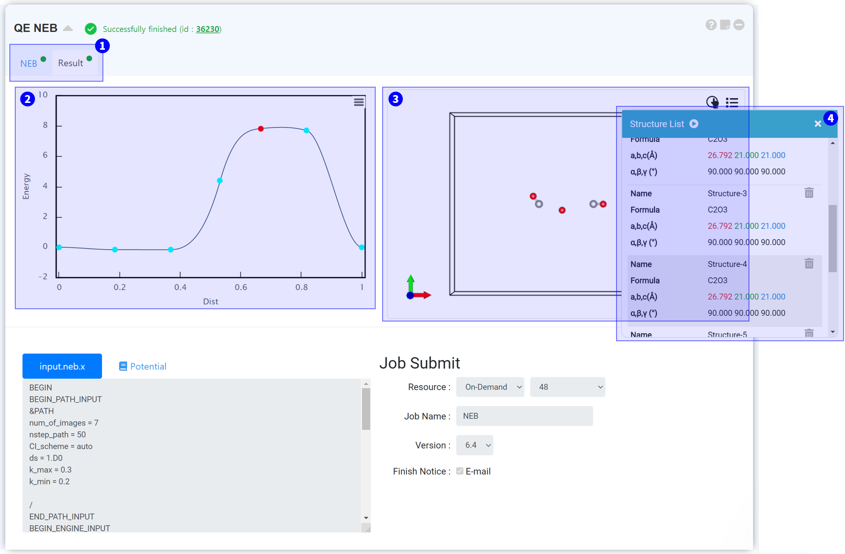
When NEB calculation is finished normally, the result tab will be displayed. Click the result tab to check the results.
NEB graph shows the energy that varies during the NEB path.
Visualizer shows a structure that varies during the NEB path.
Click the structure list icon at the ③ Visualizer upper-right to see the structure list.
In order to perform NEB calculations, you must add the initial, final images (if necessary, up to the intermediate image) to the structure list in the 'Structure Builder' connected to the 'Reaction Path (NEB)' module. For a better results, all the images should be optimized (relaxed).
See the Quantum Espresso Input description (neb.x) for a detailed explanation of the NEB input script settings.
You can select General and Manual mode in the Reaction Path (NEB) module.
It is a tool for fixing some atoms during the NEB path. The tab number means the order of the structure list in the connected structure builder. If you select atoms you want, the atoms will consider fixed during NEB calculation.
This is a link to see a list of all keywords in neb.x.
A keyword belonging &PATH namelist is the keyword to adjust the option of the NEB calculation.
It used for determining NEB path. You can copy and paste the input script which is you used to relax the structure.
The input parameters will be converted into the input script form and transferred to a cloud computing server. Please check if the script has no error.
After finishing the setting, submit the job to cloud server by referring to the Job submit section.
When NEB calculation is finished normally, the result tab will be displayed. Click the result tab to check the results.
NEB graph shows the energy that varies during the NEB path.
Visualizer shows a structure that varies during the NEB path.
Click the structure list icon at the ③ Visualizer upper-right to see the structure list.
'Phonon' is a module for phonon calculation using ph.x solver provided from Quantum Espresso.
Phonon calculation must start from 'fully relaxed structure' due to that describe interatomic vibration, therefore, it needs to perform considerably 'accurate' calculation.
It is recommended to perform phonon calculation as follows.
1. (vc-)relax calculation for primitive cell with high precision.
2. Perform phonon calculation by connecting with the Quantum Espresso module of step 1.
3. Perform the post-processing calculation.
For further information, please refer to [MatSQ Tip] Performing Phonon Calculation, Phonon examples, and Phonon webinar video.
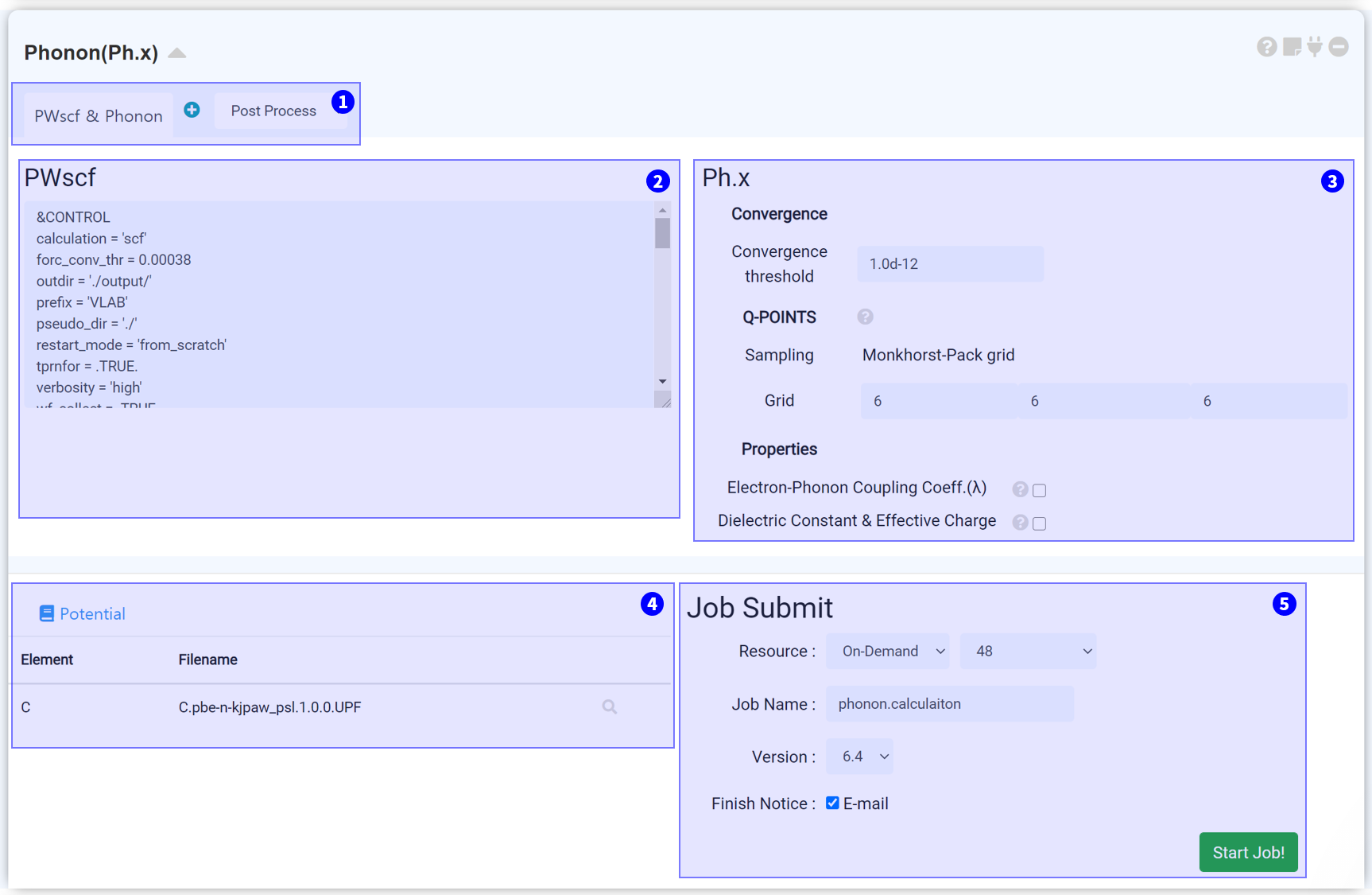
You can obtain phonon band structure and DOS graph by adding post process tab. Refer to folloiwng Post process setting for details.
This part is for SCF calculation. Basically it copies input script of connected Quantum Espresso module, and changes the calculation type to scf.
Determine the convergence threshold for phonon calculation. The default value is 1.0d-12 Ry. It is recommended if you were careful to change this value because It affects the results directly.
It is for convergence threshold and q-points in phonon calculation. The q-point should be set in the same method as the k-point, but using the same value as k-points will tremendously increase the calculation amount. Therefore, it is better to set the q-point grid smaller than the k-point.
Determine what property to obtain from phonon calculation. Electron-Phonon Coupling Coefficient (λ) is available for metal system (occupation = "smearing"), Dielectric Constant & Effective Charge is available for non-metal system (occupation = "fixed").
Set pseudopotential for calculation. It should be the same with the file used for the connected QE module.
If you have completed all the settings, set the job name and click the Start Job! button.
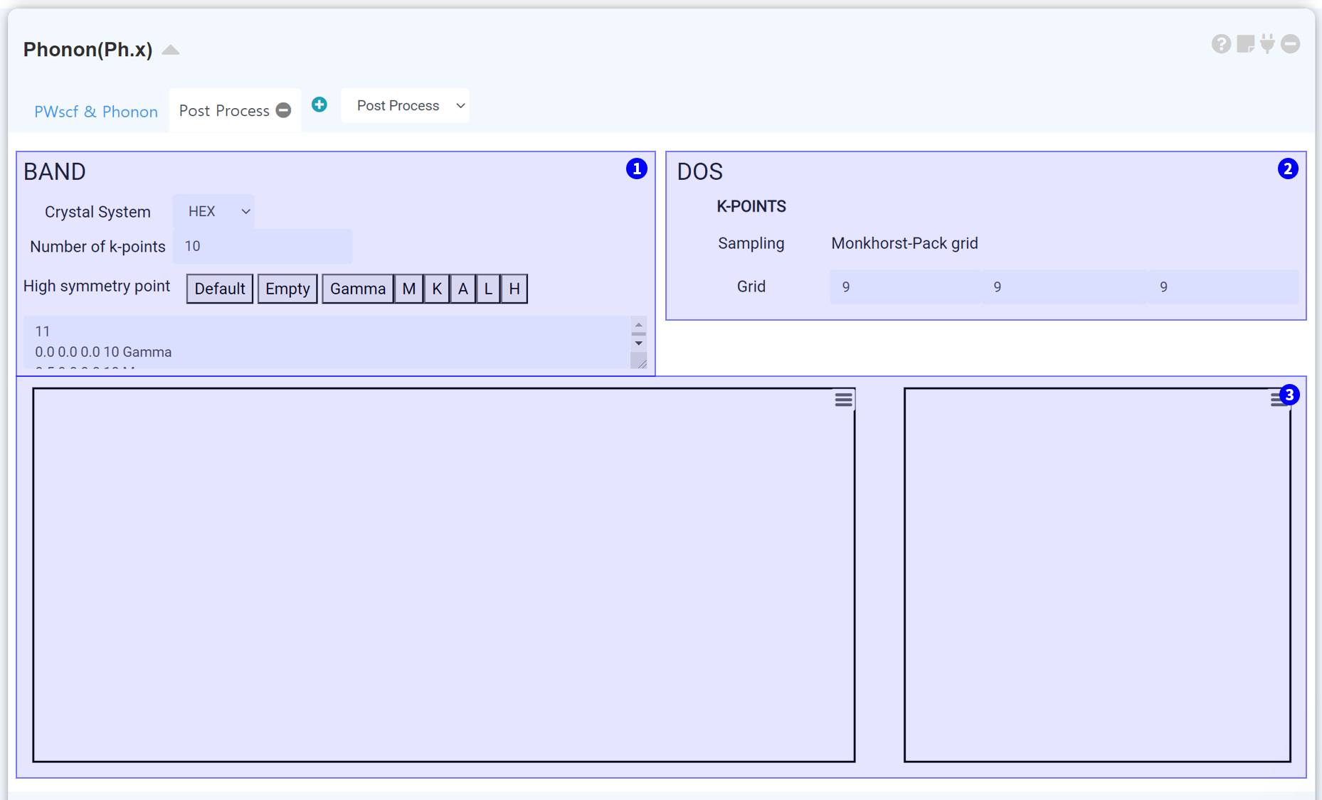
Set k-path for phonon band structure. Select appropriate crystal system, and enter the number of k-point properly. If you set the number of k-point larger, the number of k-point sampling between two high symmetry points increased.
Set the k-point grid for phonon DOS calculation.
If the calculation has been finished normally, the phonon band structure and DOS displayed in this part.
Phonon calculation must start from 'fully relaxed structure' due to that describe interatomic vibration, therefore, it needs to perform considerably 'accurate' calculation.
It is recommended to perform phonon calculation as follows.
1. (vc-)relax calculation for primitive cell with high precision.
2. Perform phonon calculation by connecting with the Quantum Espresso module of step 1.
3. Perform the post-processing calculation.
For further information, please refer to [MatSQ Tip] Performing Phonon Calculation, Phonon examples, and Phonon webinar video.
You can obtain phonon band structure and DOS graph by adding post process tab. Refer to folloiwng Post process setting for details.
This part is for SCF calculation. Basically it copies input script of connected Quantum Espresso module, and changes the calculation type to scf.
Determine the convergence threshold for phonon calculation. The default value is 1.0d-12 Ry. It is recommended if you were careful to change this value because It affects the results directly.
It is for convergence threshold and q-points in phonon calculation. The q-point should be set in the same method as the k-point, but using the same value as k-points will tremendously increase the calculation amount. Therefore, it is better to set the q-point grid smaller than the k-point.
Determine what property to obtain from phonon calculation. Electron-Phonon Coupling Coefficient (λ) is available for metal system (occupation = "smearing"), Dielectric Constant & Effective Charge is available for non-metal system (occupation = "fixed").
Set pseudopotential for calculation. It should be the same with the file used for the connected QE module.
If you have completed all the settings, set the job name and click the Start Job! button.
Set k-path for phonon band structure. Select appropriate crystal system, and enter the number of k-point properly. If you set the number of k-point larger, the number of k-point sampling between two high symmetry points increased.
Set the k-point grid for phonon DOS calculation.
If the calculation has been finished normally, the phonon band structure and DOS displayed in this part.
This module is for performing Quantum Espresso High throughput calculations. When you connect this with the structure builder module, it brings all of the structures added to the structure list at that time, and generates high throughput input scripts for the structures.
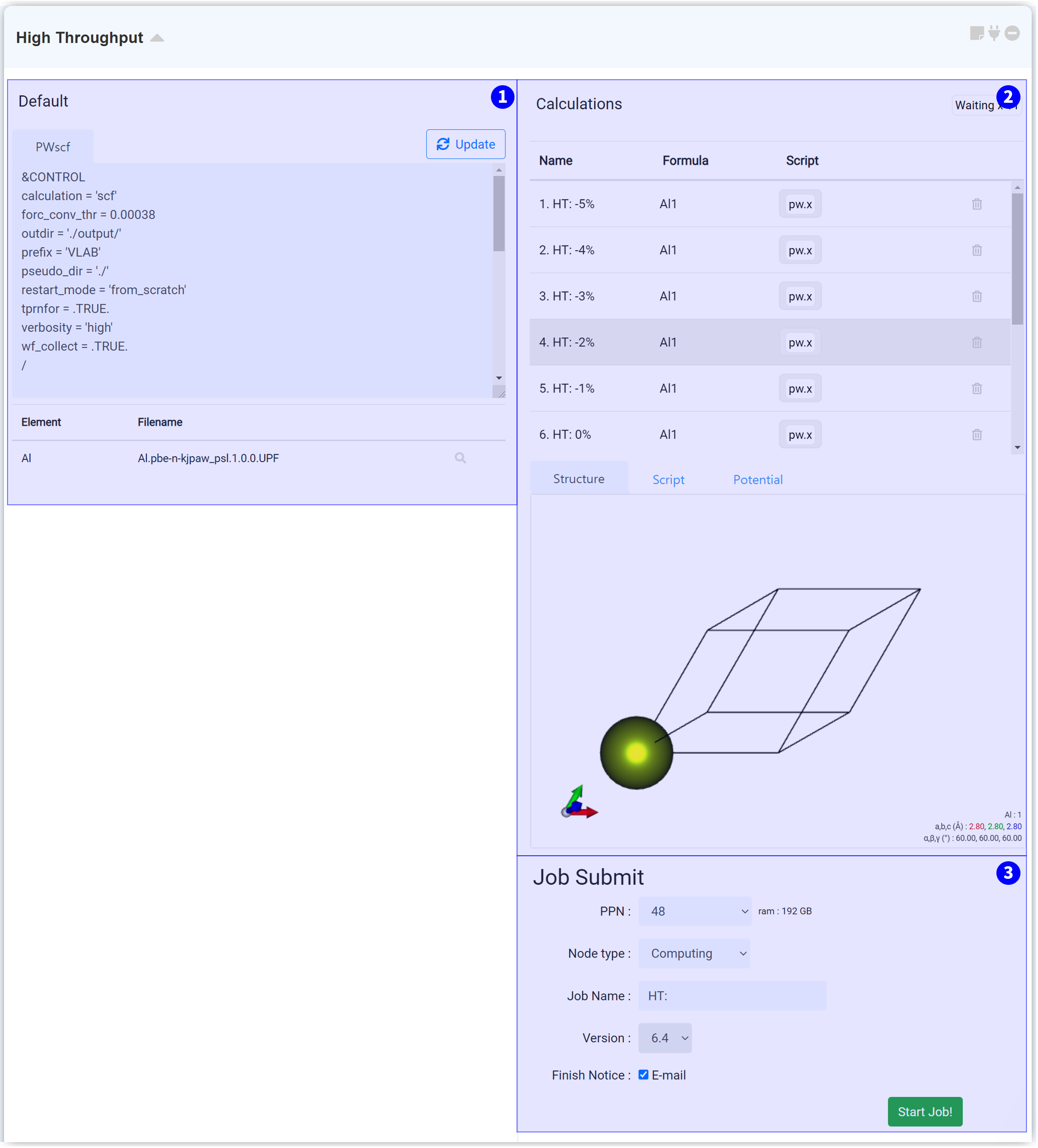
Modify and apply the entire input script and pseudopotential in this tab. For the effortless setting, paste the input script by setting it on the Quantum Espresso (General) module.
After finishing setting the desired Input script and pseudopotential, click the 'Update' button on the right-top side. Then every input script of every contained high throughput job is changed.
This part is for changing the input script and pseudopotential of each job. And also, you can check each model.
After finishing the setting, submit the job to cloud server by referring to the Job submit section.
The "SIESTA" module is a module for performing electronic structure calculation using SIESTA, a DFT-based calculation software package.
SIESTA is the same DFT-based calculation module as the “Quantum Espresso”, but there are two major differences.
Materials Square provides an intuitive graphical interface (GUI) that makes it easy to perform DFT calculations with just a few clicks without studying complex code.
Most of calculations can be performed in "General" mode to get reasonable results by simply changing the main variables such as Calculation Type, Mesh Cutoff, and K-point. In addition, for experienced users, we also provide a "Manual" mode that allows users to directly modify the script.
More information about SIESTA can be found in the SIESTA official website .
This module allows you to perform DFT-based basic calculations, recalculations, and post-processing calculations using SIESTA. The calculations that can be performed in this module are 1. Atomic/electronic structure optimization calculation, 2. Phonon calculation, and 3. AIMD calculation. Each calculation can be selected from "Calculation Type".
1. Atomic and/or electronic structures optimization
This calculation must be performed to obtain the properties of a material based on DFT. This is a calculation that finds the atomic and/or electronic configuration of the system that minimizes the total energy of the system by repeatedly adjusting the atomic positions or electron distribution state of the system. The larger the number of atoms/electrons in the system and the higher the convergence criterion, the more computational resources are required.
2. Phonon calculation
Phonon calculations are calculations that describe the vibrations between atoms. This calculation must start from a very 'stable structure' and perform very 'precise' calculations.
3. AIMD calculation
SIESTA provides Ab initio Molecular Dynamics (AIMD) calculations that simulate molecular dynamics based on quantum mechanics.
Unlike Classical MD, AIMD is based on the principles of quantum mechanics, which allows for more accurate predictions of physical and chemical properties of molecules than classical MD. However, because it is calculated by considering electronic interactions, there is a limit to the number of atoms, and it requires more computational resources than classical MD.
The MD algorithm provided by SIESTA is as follows.
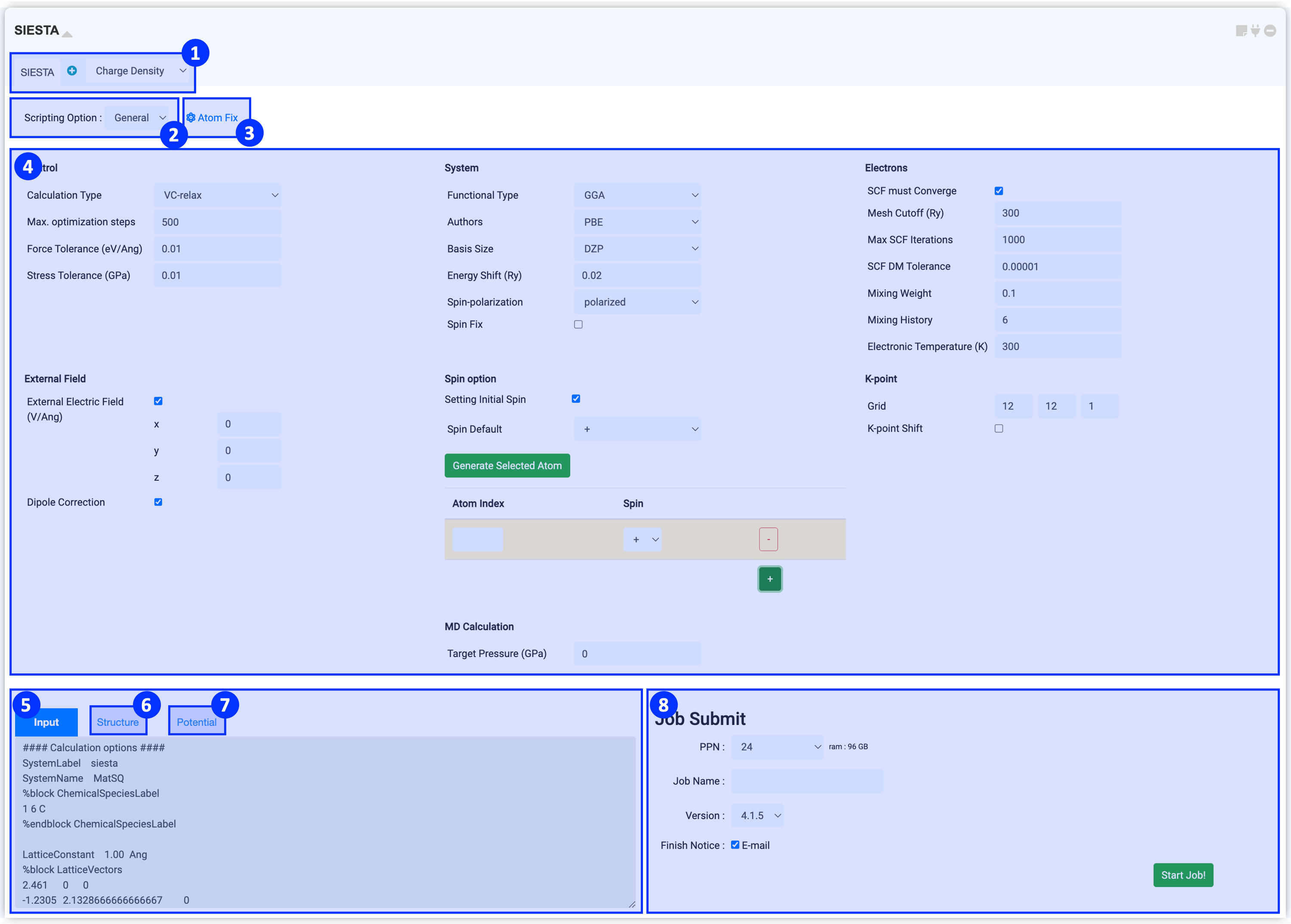
At the top of the module, you can select a solver for your calculation. In Solver region, you can find "SIESTA" solver for running basic calculation and various solvers for post-processing calculations.
SIESTA solver allows cell & atomic structure relaxation (vc-relax), atomic structure relaxation (relax), electronic structure relaxation (SCF), phonon calculation, and ab initio molecular dynamics (AIMD) calculation. For information on post-processing solvers, please refer to Post-processing calculation .
When you click the Scripting option, you can see General and Manual options. General mode is set to appropriate values for commonly used input keywords, and Manual mode can be used if user needs more keyword settings.
The SIESTA module gets the structure information from the connected Structure Builder. If you click on the coordinates of atoms in the window that opens by clicking Atom Fix, the position of the selected atom will be fixed during DFT calculation. You can easily fix an atom by selecting the atom you want to fix in Structure Builder and clicking "selected".
In SIESTA module at Materials Square, we have configured the General mode to make it easy to perform DFT calculations with just a few clicks. In General mode, we have set generally appropriate values for frequently used input keywords by default. For most calculations, reasonable results can be obtained simply by modifying the values of key keywords, but to perform highly reliable DFT simulations for use in research, such as writing papers, the values must be carefully considered and selected based on an understanding of each input keyword.
For more information, please refer to Appendix .
When you connect the SIESTA module to Structure Builder and set the input parameters, the input script and structure information are automatically created. The ⑤ Input contains the keyword setting information required for calculation, and information related to structure is written in the ⑥ Structure. This information is text that is sent to the actual server, so it is always a good idea to check that the values you set are applied correctly. If you change the option to Manual in ② Scripting Option, the ④ Input parameters will be omitted and only the Input script window will remain, and you can edit the script directly.
When performing DFT calculations, it is the pseudopotential that determines the behavior of the atoms. Therefore, before calculating, you must first set up the pseudopotential file you want to use. For information on setting the pseudopotential file, please refer to "Pseudopotential setting".
⑦ Pseudopotential tab shows the files that have been set up. Press the magnifying glass button to see the list of available pseudopotentials. Materials Square database uses pseudopotential file downloaded from NNIN Virtual Vault for Pseudopotentials by default. For more information about pseudopotential, please refer to the Pseudopotential Files .
If you have completed all settings in steps ①~⑦, you are ready to submit your job. Please refer to the Job submit document to start the calculation process.
If you connect a new SIESTA module to the previous SIESTA module that finished calculation, you can perform a restart calculation that continues the calculation from the point where the calculation ended. However, you cannot restart from a calculation in which an error occurred. Please refer to "Trouble shooting" for a description of the error.
Restart calculation is to load the input parameter and the structure information of the last step from the calculation performed in the previous calculation. When a new SIESTA module is connected to a previous SIESTA module, the input parameters and final structure information are copied to the new module.
Restart calculation is useful in the following cases:
1. When the message "Structure is not relaxed" is displayed: : This is a case where the calculation has progressed to the number of steps (Max Iteration Step) set in the atomic structure optimization process but has not reached the convergence force tolerance value. In this case, it is recommended to load the final structure and use the same input parameters but increase the number of Max Iteration Steps and recalculate in case optimization is not completed again.
2. When performing post-processing calculation : This calculation is to perform the post-processing calculation for electronic structure analysis from the optimized atomic structure. To calculate DOS, Band Structures, and Optical Properties, change the Calculation Type to SCF and add the post-processing solver you want to analyze.
Information about the input parameters of each calculation method can be found in "Appendix".
Post-processing calculations are performed after the calculation through the "SIESTA" solver is completed and can be obtained by adding the post-processing solver for which you want to calculate.
SIESTA is the same DFT-based calculation module as the “Quantum Espresso”, but there are two major differences.
Materials Square provides an intuitive graphical interface (GUI) that makes it easy to perform DFT calculations with just a few clicks without studying complex code.
Most of calculations can be performed in "General" mode to get reasonable results by simply changing the main variables such as Calculation Type, Mesh Cutoff, and K-point. In addition, for experienced users, we also provide a "Manual" mode that allows users to directly modify the script.
More information about SIESTA can be found in the SIESTA official website .
This module allows you to perform DFT-based basic calculations, recalculations, and post-processing calculations using SIESTA. The calculations that can be performed in this module are 1. Atomic/electronic structure optimization calculation, 2. Phonon calculation, and 3. AIMD calculation. Each calculation can be selected from "Calculation Type".
1. Atomic and/or electronic structures optimization
This calculation must be performed to obtain the properties of a material based on DFT. This is a calculation that finds the atomic and/or electronic configuration of the system that minimizes the total energy of the system by repeatedly adjusting the atomic positions or electron distribution state of the system. The larger the number of atoms/electrons in the system and the higher the convergence criterion, the more computational resources are required.
2. Phonon calculation
Phonon calculations are calculations that describe the vibrations between atoms. This calculation must start from a very 'stable structure' and perform very 'precise' calculations.
3. AIMD calculation
SIESTA provides Ab initio Molecular Dynamics (AIMD) calculations that simulate molecular dynamics based on quantum mechanics.
Unlike Classical MD, AIMD is based on the principles of quantum mechanics, which allows for more accurate predictions of physical and chemical properties of molecules than classical MD. However, because it is calculated by considering electronic interactions, there is a limit to the number of atoms, and it requires more computational resources than classical MD.
The MD algorithm provided by SIESTA is as follows.
-
(1) Verlet (NVE): Standard Verlet algorithm MD
(2) Nose (NVT): temperature controlled by means of a Nosé thermostat
(3) ParrinelloRahman (NPE): pressure controlled by the Parrinello-Rahman method
(4) Nose-ParrinelloRahman (NPT): annealing to a desired temperature and/or pressure
(5) Anneal: annealing to a desired temperature and/or pressure
At the top of the module, you can select a solver for your calculation. In Solver region, you can find "SIESTA" solver for running basic calculation and various solvers for post-processing calculations.
SIESTA solver allows cell & atomic structure relaxation (vc-relax), atomic structure relaxation (relax), electronic structure relaxation (SCF), phonon calculation, and ab initio molecular dynamics (AIMD) calculation. For information on post-processing solvers, please refer to Post-processing calculation .
When you click the Scripting option, you can see General and Manual options. General mode is set to appropriate values for commonly used input keywords, and Manual mode can be used if user needs more keyword settings.
The SIESTA module gets the structure information from the connected Structure Builder. If you click on the coordinates of atoms in the window that opens by clicking Atom Fix, the position of the selected atom will be fixed during DFT calculation. You can easily fix an atom by selecting the atom you want to fix in Structure Builder and clicking "selected".
In SIESTA module at Materials Square, we have configured the General mode to make it easy to perform DFT calculations with just a few clicks. In General mode, we have set generally appropriate values for frequently used input keywords by default. For most calculations, reasonable results can be obtained simply by modifying the values of key keywords, but to perform highly reliable DFT simulations for use in research, such as writing papers, the values must be carefully considered and selected based on an understanding of each input keyword.
For more information, please refer to Appendix .
When you connect the SIESTA module to Structure Builder and set the input parameters, the input script and structure information are automatically created. The ⑤ Input contains the keyword setting information required for calculation, and information related to structure is written in the ⑥ Structure. This information is text that is sent to the actual server, so it is always a good idea to check that the values you set are applied correctly. If you change the option to Manual in ② Scripting Option, the ④ Input parameters will be omitted and only the Input script window will remain, and you can edit the script directly.
When performing DFT calculations, it is the pseudopotential that determines the behavior of the atoms. Therefore, before calculating, you must first set up the pseudopotential file you want to use. For information on setting the pseudopotential file, please refer to "Pseudopotential setting".
⑦ Pseudopotential tab shows the files that have been set up. Press the magnifying glass button to see the list of available pseudopotentials. Materials Square database uses pseudopotential file downloaded from NNIN Virtual Vault for Pseudopotentials by default. For more information about pseudopotential, please refer to the Pseudopotential Files .
If you have completed all settings in steps ①~⑦, you are ready to submit your job. Please refer to the Job submit document to start the calculation process.
If you connect a new SIESTA module to the previous SIESTA module that finished calculation, you can perform a restart calculation that continues the calculation from the point where the calculation ended. However, you cannot restart from a calculation in which an error occurred. Please refer to "Trouble shooting" for a description of the error.
Restart calculation is to load the input parameter and the structure information of the last step from the calculation performed in the previous calculation. When a new SIESTA module is connected to a previous SIESTA module, the input parameters and final structure information are copied to the new module.
Restart calculation is useful in the following cases:
- When the message "Structure is not relaxed" is displayed.
- When performing post-processing calculations such as DOS, Bands, optical, phonon, etc.
1. When the message "Structure is not relaxed" is displayed: : This is a case where the calculation has progressed to the number of steps (Max Iteration Step) set in the atomic structure optimization process but has not reached the convergence force tolerance value. In this case, it is recommended to load the final structure and use the same input parameters but increase the number of Max Iteration Steps and recalculate in case optimization is not completed again.
2. When performing post-processing calculation : This calculation is to perform the post-processing calculation for electronic structure analysis from the optimized atomic structure. To calculate DOS, Band Structures, and Optical Properties, change the Calculation Type to SCF and add the post-processing solver you want to analyze.
Information about the input parameters of each calculation method can be found in "Appendix".
Post-processing calculations are performed after the calculation through the "SIESTA" solver is completed and can be obtained by adding the post-processing solver for which you want to calculate.
- Add the SIESTSA module, and in ① Solver, click on the postprocessing solver (DOS, charge density, and etc.) to obtain the desired data. Then, press the + button to add a new solver tab next to SIESTA. Post-processing solver can add as much data as you want to obtain.
- For Phonon calculations, the Phonon post-processing tab is automatically added.
- Pressing the Start Job! button will run the SIESTA calculation and all the added post-processing jobs.
The potential file of the SIESTA module basically uses Norm-Conserving PP. Materials Square provides potential files for the well-known CA(=PZ) and PBE functionals.
However, we are not responsible for its suitability for your specific system.
We recommend that pseudopotentials and basis sets be tested and used in well-known situations before using them in your system. Especially if you are using a different potential type, please be sure to upload a file that you have personally created and test it before using it.
We recommend that pseudopotentials and basis sets be tested and used in well-known situations before using them in your system. Especially if you are using a different potential type, please be sure to upload a file that you have personally created and test it before using it.
- Virtual Vault : These are potential files downloaded from Virtual Vault Database recommended for non-academic users on the SIESTA homepage.
- MatSQ: These are relativistic type potential files created by the MatSQ Team using ATOM. To calculate SOC, you must use this potential file or use a relativistic type of potential file that you upload yourself.
- User upload: You can upload a user-created potential and use it. If your potential file is set to semicore state, %block PAO.Basis must be set manually in input file.
The GAMESS module is the tool to perform electronic structure calculation using GAMESS (US), an open-source software for ab initio molecular quantum chemistry. MatSQ provides an intuitive graphical interface (GUI) that makes it easy to perform DFT calculations without having to deeply study how to use the software. Specifically,'Scripting Options: Template' allows you to create an input script with a few button clicks. Of course, MatSQ also provides a manual option for experienced users who can directly modify the script.
For the more detail for GAMESS, please refer to the www.msg.chem.iastate.edu/gamess/
To find description for the GAMESS input parameters, please refer to the To learn GAMESS input section.
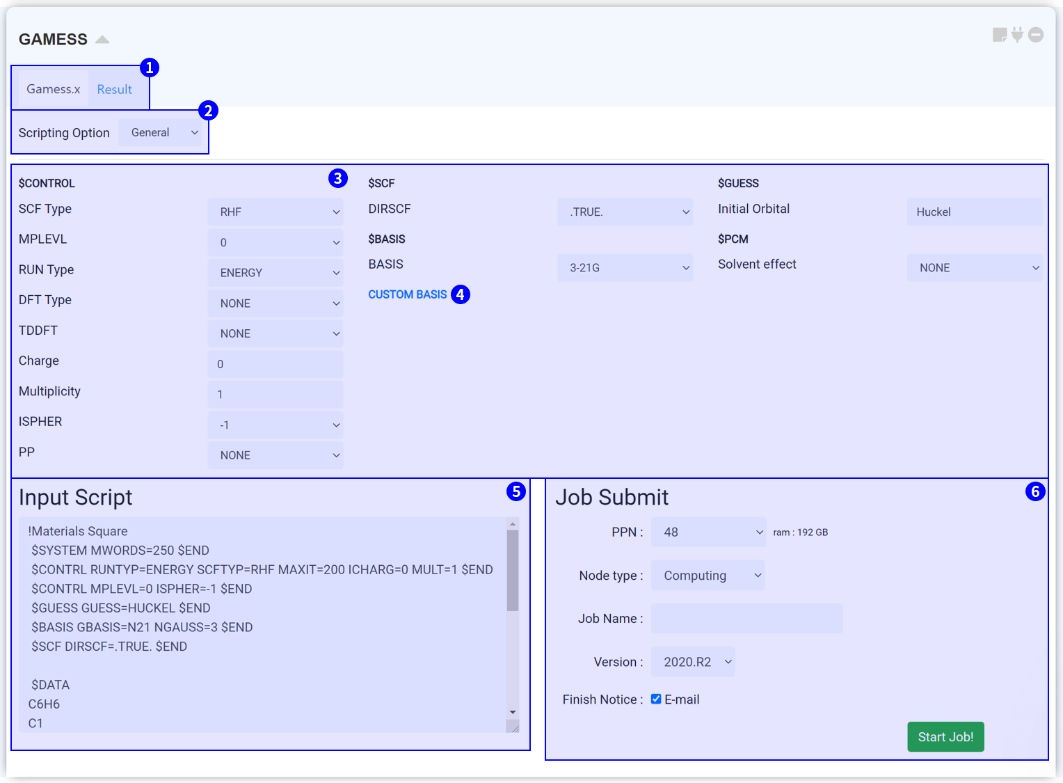
On the top side, you can see the two tabs. At the 'Gamess.x' tab, you can set the input script for conducting GAMESS. After finishing the calculation, click the 'Result' tab to check the calculation results.
Press the 'Scripting Option' to view 'Template,' 'General,' and 'Manual' options. The 'Template' is a good option for those who are not familiar with the keyword settings in GAMESS. In the Template, answer the three questions to set the input script.
MatSQ makes it easy to perform DFT calculations with just a few clicks. The default values of the GAMESS module are set as commonly proper values, therefore, you can obtain good results by changing only major keywords. However, the values should be carefully considered and selected based on an understanding of each input parameter to perform reliable DFT simulations for advanced use such as for research and papers. For the Input parameter description, please refer to the GAMESS Manual or To learn GAMESS input section.
The GAMESS does not provide all of the built-in basis set used in chemical calculations. Especially, structures including heavy atoms often do not have an adequate built-in basis set. For this cases, you should find and apply the custom basis set. You can refer to or download various basis sets from the Basis Set Exchange (BSE).
An input script is created when the GAMESS module is connected to Structure Builder, and input parameters are set. The input script is a text sent to the cloud server, that has structure information and keyword setting information. Therefore, it is recommended that you always ensure the values you set are correctly applied. When you change the option to Manual in ② Scripting Option, the ③ Input Parameters section is omitted. Only the Input Script window remains to allow you to modify the script manually. When you modify text in the Input Script window, the mode automatically changes to Manual.
After finishing the setting, submit the job to cloud server by referring to the Job submit section.
If you connect a new GAMESS module to the QE module that has finished the calculation, you can proceed with further calculations from the last point with “restart.” Especially, you can restart the calculation that has been interrupted by the user request. But please note that the errored calculation cannot be restarted.
For the more detail for GAMESS, please refer to the www.msg.chem.iastate.edu/gamess/
To find description for the GAMESS input parameters, please refer to the To learn GAMESS input section.
On the top side, you can see the two tabs. At the 'Gamess.x' tab, you can set the input script for conducting GAMESS. After finishing the calculation, click the 'Result' tab to check the calculation results.
Press the 'Scripting Option' to view 'Template,' 'General,' and 'Manual' options. The 'Template' is a good option for those who are not familiar with the keyword settings in GAMESS. In the Template, answer the three questions to set the input script.
- Target property: Select what data you want to obtain. The input script is changed appropriately according to match the answer.
- Energy/Optimization/Vibration: It determines whether perform the geometry optimization, and whether calculate the vibrational properties.
- Option: It determines whether considers what additional option to the calculation.
MatSQ makes it easy to perform DFT calculations with just a few clicks. The default values of the GAMESS module are set as commonly proper values, therefore, you can obtain good results by changing only major keywords. However, the values should be carefully considered and selected based on an understanding of each input parameter to perform reliable DFT simulations for advanced use such as for research and papers. For the Input parameter description, please refer to the GAMESS Manual or To learn GAMESS input section.
The GAMESS does not provide all of the built-in basis set used in chemical calculations. Especially, structures including heavy atoms often do not have an adequate built-in basis set. For this cases, you should find and apply the custom basis set. You can refer to or download various basis sets from the Basis Set Exchange (BSE).
An input script is created when the GAMESS module is connected to Structure Builder, and input parameters are set. The input script is a text sent to the cloud server, that has structure information and keyword setting information. Therefore, it is recommended that you always ensure the values you set are correctly applied. When you change the option to Manual in ② Scripting Option, the ③ Input Parameters section is omitted. Only the Input Script window remains to allow you to modify the script manually. When you modify text in the Input Script window, the mode automatically changes to Manual.
After finishing the setting, submit the job to cloud server by referring to the Job submit section.
If you connect a new GAMESS module to the QE module that has finished the calculation, you can proceed with further calculations from the last point with “restart.” Especially, you can restart the calculation that has been interrupted by the user request. But please note that the errored calculation cannot be restarted.
The ‘GAMESS-IRC’ module performs intrinsic reaction coordinate (IRC) calculations using GAMESS (US), an open-source software for ab initio molecular quantum chemistry.
You should prepare the GAMESS module set up with the ‘RUNTYP=SADPOINT’ option. The GAMESS-IRC module should then be connected to the GAMESS module, with only one selected imaginary frequency (saddle point).
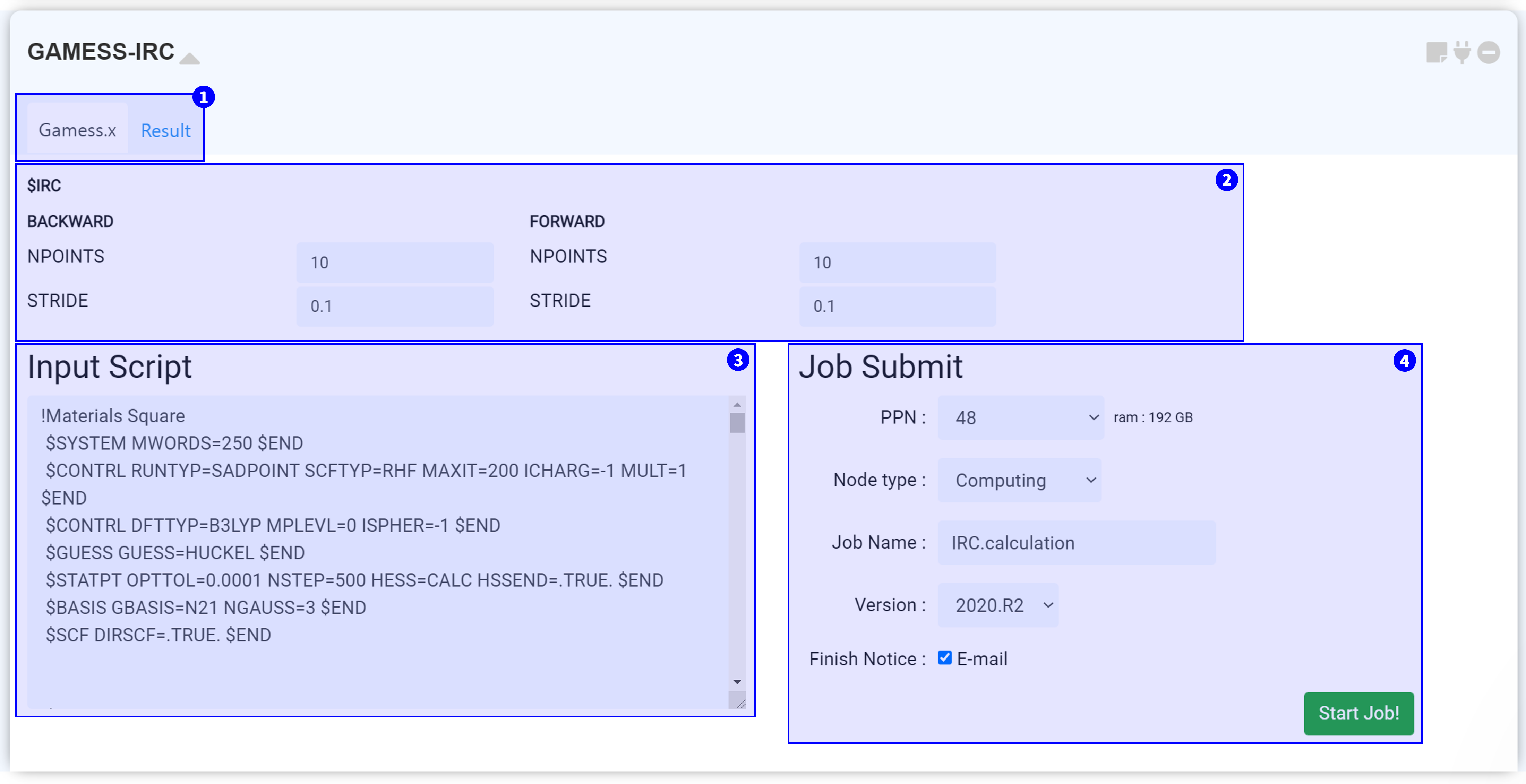
On the top side, you can see the two tabs. Under the 'Gamess.x' tab, you can set the input script for executing GAMESS-IRC. After finishing the calculation, click the 'Result' tab to check the calculation results.
MatSQ makes it easy to perform DFT calculations with just a few clicks. The default values of the GAMESS module are set as common proper values, therefore, you can obtain good results by changing only major keywords. However, the values should be carefully considered and selected based on an understanding of each input parameter to perform reliable DFT simulations for advanced use, such as for research and for publishing papers. For the Input parameter description, please refer to the GAMESS Manual.
The input script is created when the GAMESS-IRC module is connected to the GAMESS module which performed the saddle point calculation (RUNTYP=SADPOINT). This input script is generated from the set ② Input parameter. It is recommended that you always ensure the values you set are correctly applied.
After finishing setting-up the calculation, submit the job to the cloud server by referring to the Job submit section.
You should prepare the GAMESS module set up with the ‘RUNTYP=SADPOINT’ option. The GAMESS-IRC module should then be connected to the GAMESS module, with only one selected imaginary frequency (saddle point).
On the top side, you can see the two tabs. Under the 'Gamess.x' tab, you can set the input script for executing GAMESS-IRC. After finishing the calculation, click the 'Result' tab to check the calculation results.
MatSQ makes it easy to perform DFT calculations with just a few clicks. The default values of the GAMESS module are set as common proper values, therefore, you can obtain good results by changing only major keywords. However, the values should be carefully considered and selected based on an understanding of each input parameter to perform reliable DFT simulations for advanced use, such as for research and for publishing papers. For the Input parameter description, please refer to the GAMESS Manual.
The input script is created when the GAMESS-IRC module is connected to the GAMESS module which performed the saddle point calculation (RUNTYP=SADPOINT). This input script is generated from the set ② Input parameter. It is recommended that you always ensure the values you set are correctly applied.
After finishing setting-up the calculation, submit the job to the cloud server by referring to the Job submit section.
The ‘GAMESS-NEB’ module is for performing Nudged Elastic Band (NEB) calculations using GAMESS (US), an open-source software for ab initio molecular quantum chemistry.
In order to perform NEB calculations, you must connect the module to the Structure Builder module, which have two or more structures. Add the initial and final images (with intermediate images, if necessary) to the structure list in the 'Structure Builder' module. For better results, all the images should be initially optimized (relaxed).
The atom order of all molecules must be the same. The atom order can be checked in the ‘Edit’ menu.
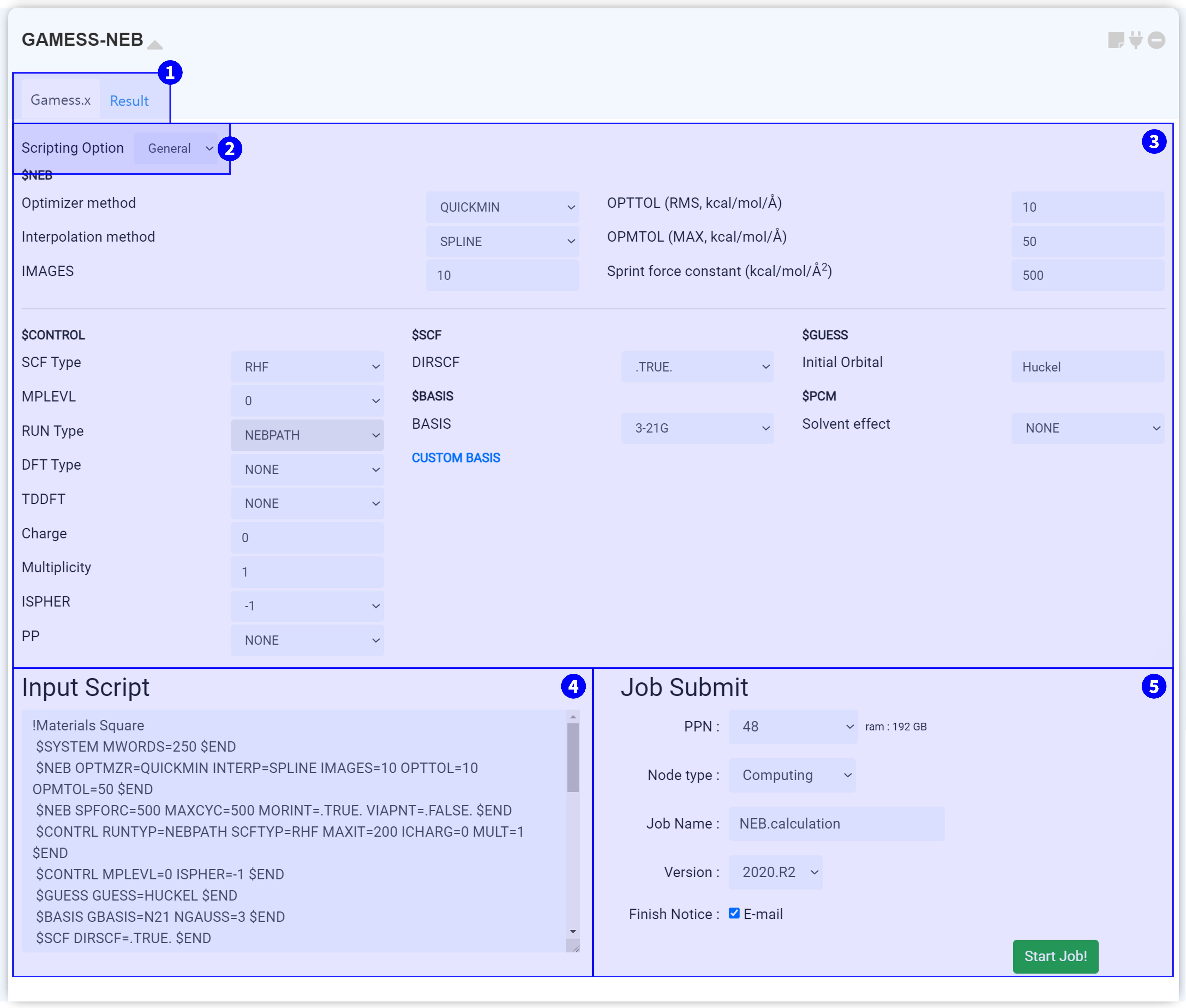
On the top side, you can see the two tabs. Under the ‘Gamess.x’ tab, you can set the input script for conducting the GAMESS-NEB calculation. After finishing the calculation, click the ‘Result’ tab to check the calculation results.
You can select either the “General” or “Manual” mode under the “Scripting” option.
The input setting window of the GAMESS-NEB module can be divided into two parts. In the $NEB group, you can modify the NEB calculation options. Moreover, you can adjust the convergence options in $CONTROL and in other groups. For the Input parameter description, please refer to the GAMESS Manual.
The input script is created when the GAMESS-NEB module is connected to the Structure builder module with Initial/Intermediate(optional)/Final images. This input script is generated from the set ② Input parameter. It is recommended that you always ensure the values you set are correctly applied. When you change the option to “Manual” in ② “Scripting Option”, the ③ “Input Parameters” section is omitted. Only the “Input Script” window remains to modify the script manually. When you modify the text in the “Input Script” window, the mode automatically changes to “Manual”.
After finishing setting-up the calculation, submit the job to the cloud server by referring to the Job submit section.
In order to perform NEB calculations, you must connect the module to the Structure Builder module, which have two or more structures. Add the initial and final images (with intermediate images, if necessary) to the structure list in the 'Structure Builder' module. For better results, all the images should be initially optimized (relaxed).
The atom order of all molecules must be the same. The atom order can be checked in the ‘Edit’ menu.
On the top side, you can see the two tabs. Under the ‘Gamess.x’ tab, you can set the input script for conducting the GAMESS-NEB calculation. After finishing the calculation, click the ‘Result’ tab to check the calculation results.
You can select either the “General” or “Manual” mode under the “Scripting” option.
The input setting window of the GAMESS-NEB module can be divided into two parts. In the $NEB group, you can modify the NEB calculation options. Moreover, you can adjust the convergence options in $CONTROL and in other groups. For the Input parameter description, please refer to the GAMESS Manual.
The input script is created when the GAMESS-NEB module is connected to the Structure builder module with Initial/Intermediate(optional)/Final images. This input script is generated from the set ② Input parameter. It is recommended that you always ensure the values you set are correctly applied. When you change the option to “Manual” in ② “Scripting Option”, the ③ “Input Parameters” section is omitted. Only the “Input Script” window remains to modify the script manually. When you modify the text in the “Input Script” window, the mode automatically changes to “Manual”.
After finishing setting-up the calculation, submit the job to the cloud server by referring to the Job submit section.
GAMESS-BDE module is for Bond Dissociation Energy (BDE) calculations using GAMESS (US), an open-source software for ab initio molecular quantum chemistry. The GAMESS-BDE module must be connected to the GAMESS module that has completed the structural optimization calculations.
You need to connect to the GAMESS module that performed the Hessian calculations to obtain not only energetics but also thermodynamic information.
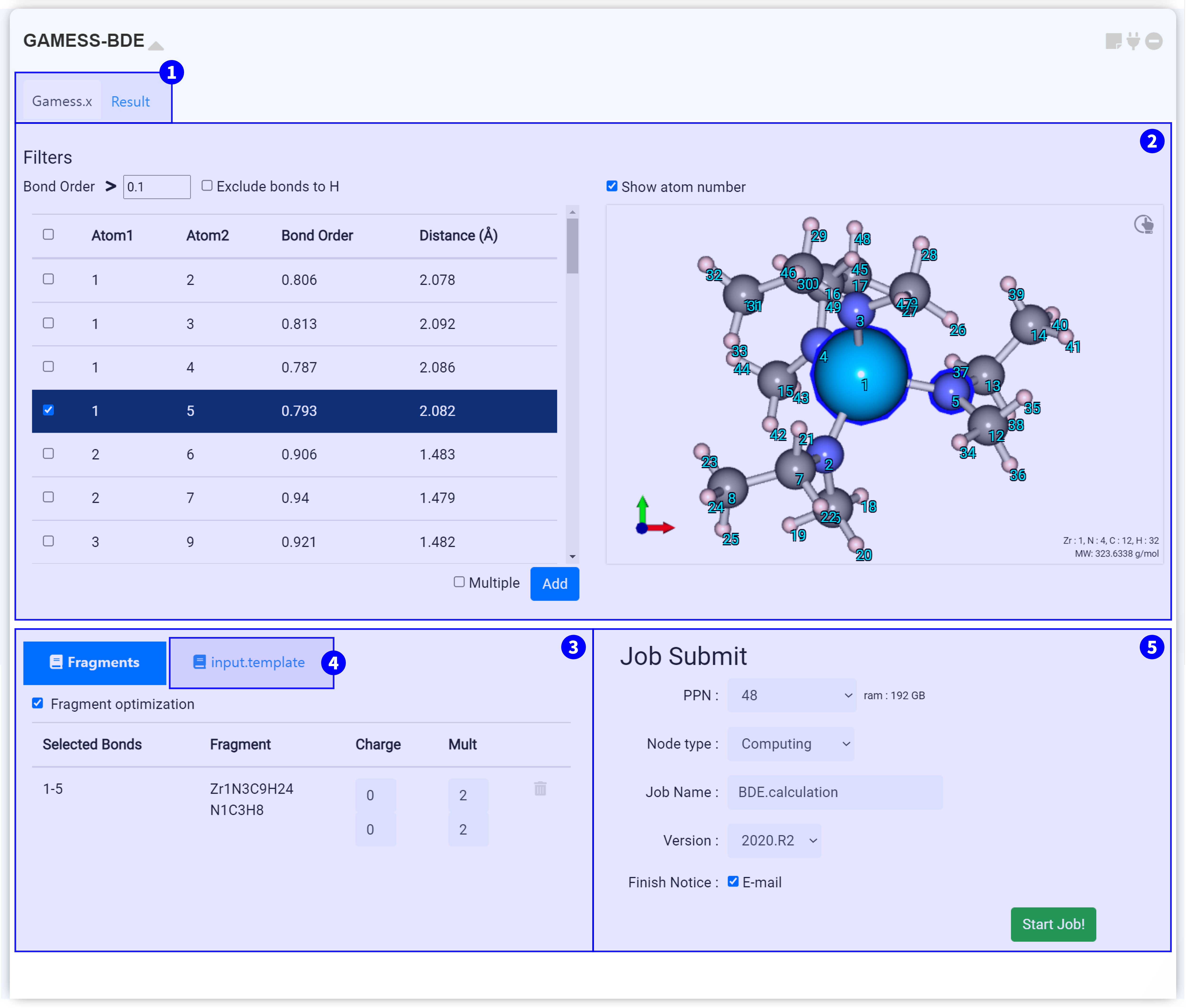
On the top side, you can see the two tabs. Under the ‘Gamess.x’ tab, you can set the input script for conducting the GAMESS-BDE calculation. After finishing the calculation, click the ‘Result’ tab to check the calculation results.
You can check the bond order and distance between atoms. Modify the ‘Bond order’ value at the top of the list to display only bonds with a bond order greater than or equal to the set value. You can also decide whether to show hydrogen bonds via the ‘Exclude bonds to H’ checkbox.
Select a bond from the list on the left hand side . Then, in the Visualizer on the right hand side , atoms of the selected bond are marked with a blue border. You can display the index number of an atom by selecting 'Show atom number' at the top of the Visualizer. Select the combination you want to create a Fragment for, and click the button to add it.
Select the 'Multiple' options to create fragments by breaking two or more bonds. After that, you can click the button to check the Fragment in color.
You can check the list of created Fragments. When you click the list, each fragment is displayed in color in the top right visualizer.
The input script is created when you set the ‘Fragment’. It is recommended that you always ensure the values you set are correctly applied.
After finishing setting-up the calculation, submit the job to the cloud server by referring to the “ Job submit ” section.
Crystal Graph Convolutional Neural Network (CGCNN) is the most successful prediction model for the materials science field combined with the machine learning approach. You may predict the various material properties, such as formation energy, bandgap, bulk/shear moduli, Poisson’s ratio, etc., through the material structure as an input.
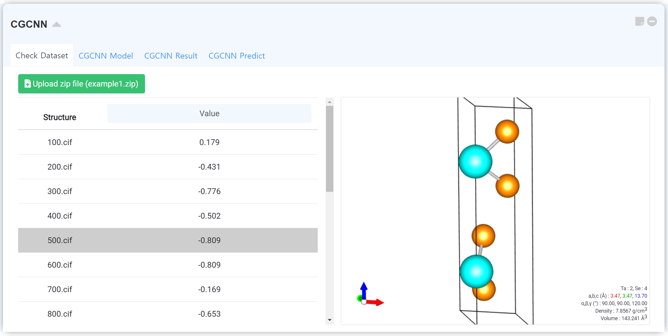
You can upload and check the training dataset in “Check Dataset” tab. Click the Upload zip file button to upload the database zip file.
1) “Zip file” consists of two parts, structure files (cif format) and property files (id_prop.csv).
2) “id_props.csv” should includes structure name (1st column, e.g. mp-100, mp-101, mp-102 …) and desired property (2nd column, e.g. 1.13, 1.42, 2.43, 1.22 …) value.
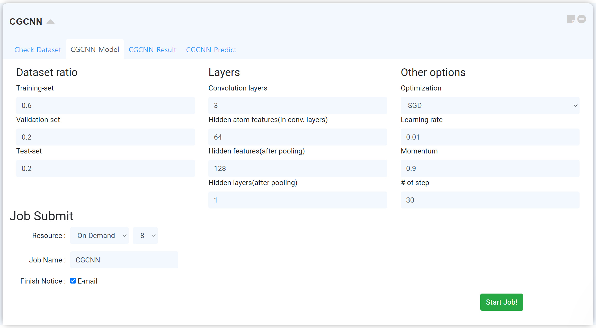
This part is for making your own machine-learning model. You can design your own machine learning model, from how to make the machine learning model by determining how to distribute the learning data and test data, to adjusting various hyper-parameters, and the optimizing method for learning. It consists of Dataset ratio, Layers, related to the network, Other options, related to optimizing.
After finishing the setting, submit the job by referring Job submit section.
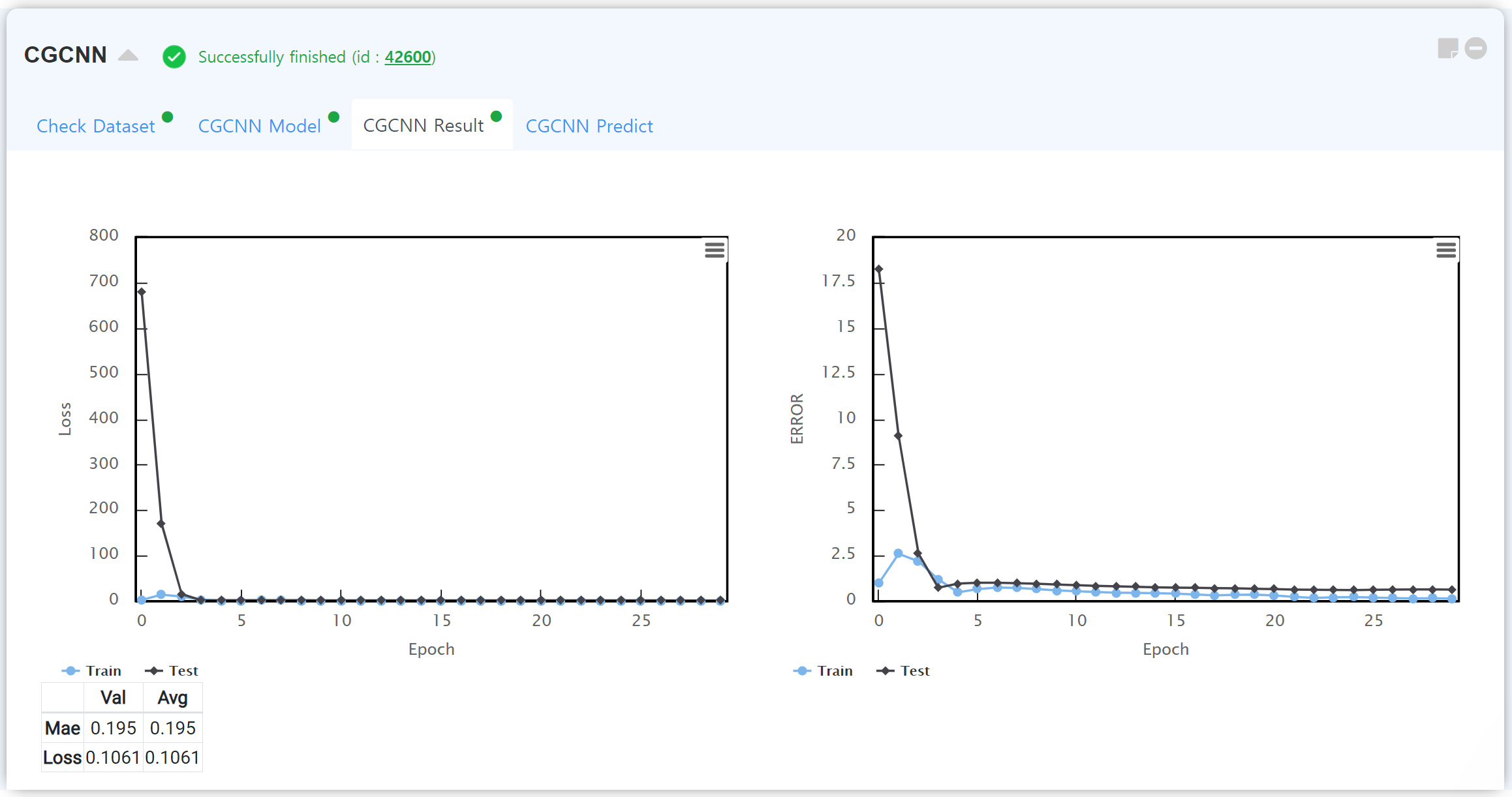
After finishing the calculation, “CGCNN Result” tab shows the accuracy of the your own CGCNN model.
You can check the value of loss function with the learning/test data as a function of epoch. Generally, the accuracy of the learning data is higher than the test data. But if the accuracy of the learning data is too high, you should consider overfitting issue.
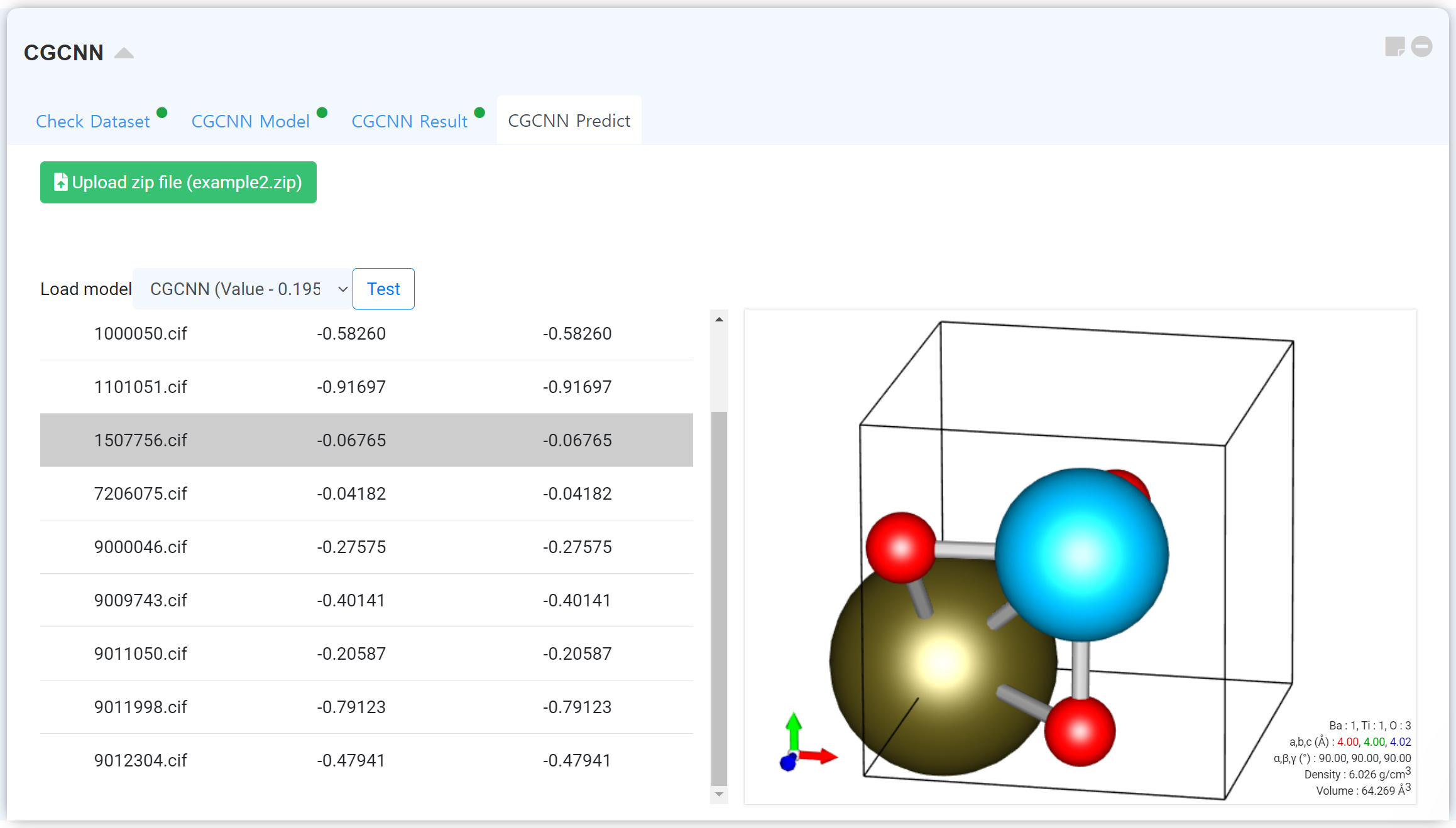
After finishing the learning, “CGCNN Predict” tab enables loading the calculated module to predict the properties of uploaded other structures. Click the Upload zip file button to upload the database zip file.
“Zip File” should include structure files (cif format) only.
You need to connect to the GAMESS module that performed the Hessian calculations to obtain not only energetics but also thermodynamic information.
On the top side, you can see the two tabs. Under the ‘Gamess.x’ tab, you can set the input script for conducting the GAMESS-BDE calculation. After finishing the calculation, click the ‘Result’ tab to check the calculation results.
You can check the bond order and distance between atoms. Modify the ‘Bond order’ value at the top of the list to display only bonds with a bond order greater than or equal to the set value. You can also decide whether to show hydrogen bonds via the ‘Exclude bonds to H’ checkbox.
Select a bond from the list on the left hand side . Then, in the Visualizer on the right hand side , atoms of the selected bond are marked with a blue border. You can display the index number of an atom by selecting 'Show atom number' at the top of the Visualizer. Select the combination you want to create a Fragment for, and click the button to add it.
Select the 'Multiple' options to create fragments by breaking two or more bonds. After that, you can click the button to check the Fragment in color.
You can check the list of created Fragments. When you click the list, each fragment is displayed in color in the top right visualizer.
The input script is created when you set the ‘Fragment’. It is recommended that you always ensure the values you set are correctly applied.
After finishing setting-up the calculation, submit the job to the cloud server by referring to the “ Job submit ” section.
Materials Square offers template modules to use LAMMPS easily. You can set the initial conditions to start the simulation with just a few clicks. All parameters of the template module are optimized for the calculation. Also, you can perform your unique simulation by adjusting 'Forcefield', 'Ensemble', 'Temperature', 'Simulation time'.
- Select the module to appropriate for the desired data.
- Set the initial parameters for the simulation. For the detail, please refer to the next 'Template details' section.
- Start the calculation by referring the Job submit section.
- Check the results on the 'Analysis' tab after finishing the simulation. For the detail, please refer to the next 'Template details' section.
- Thermalization
- Tg/CTE
- Elastic properties
- Dielectric constant
- Solubility parameter
- Viscosity (EMD)
- Viscosity (NEMD)
"Cascade" module enables to perform irradiation damage simulation. Cascade simulation is also called as collision cascade. Radiation damage simulation can be described/calculated by the atomic collision cascade, which calculates the structure variations on the high-energy atom (PKA) irradiated.
Cascade simulation needs massive model. So the model is made in the LAMMPS (CAS) module by determining the model size, instead of modeling that directly in the structure builder module. Therefore, connect the module to the structure builder module which modeled the unit cell to perform cascade simulation with LAMMPS (CAS) module.
The Primary Knock-on Atom (PKA) will be selected as the atom of origin (0, 0, 0).
Cascade simulation progresses along to the following steps.
The set total simulation time is divided into cascade and relaxation steps. However, as the time steps have changed, the total number of steps will change.
After the job has finished, click 'Update' button to update the job status. Then you can see the results at the 'Analysis' tab.
The 'Analysis' tab of the LAMMPS (CAS) module consists of Movie module and graph module. You can check the trajectory in the Movie module, and the changing number of defects at the graph of the bottom.
Cascade simulation needs massive model. So the model is made in the LAMMPS (CAS) module by determining the model size, instead of modeling that directly in the structure builder module. Therefore, connect the module to the structure builder module which modeled the unit cell to perform cascade simulation with LAMMPS (CAS) module.
The Primary Knock-on Atom (PKA) will be selected as the atom of origin (0, 0, 0).
- Select the appropriate forcefield for the system.
- Determine the size of the simulation model.
Be careful about the size of the system. The PKA might be returned to origin due to the PBC, if the system is too small, and the calculation time tremendously increase if the system is too big. - Set the PKA Direction.
Click button to set the vector ramdomly. - Set the temperature for Thermailization.
- Determine the total simulation time.
- Set a job name and click 'Start Job!' button to start the calculation.
Cascade simulation progresses along to the following steps.
- Relaxation
- Thermalization
- Cascade : NVE 1
(Velocity set, timestep 0.01 fs) - Relaxation : NVE 2
(timestep 0.03 fs)
The set total simulation time is divided into cascade and relaxation steps. However, as the time steps have changed, the total number of steps will change.
After the job has finished, click 'Update' button to update the job status. Then you can see the results at the 'Analysis' tab.
The 'Analysis' tab of the LAMMPS (CAS) module consists of Movie module and graph module. You can check the trajectory in the Movie module, and the changing number of defects at the graph of the bottom.
"EOS" module enables to calculate the equation of state. You may get some basic geometric properties, such as the ground-state volume and its energy of the system and bulk modulus, from the short and easy EOS calculation. Connect this to the structure builder module which modeled the unit cell.
After the job has finished, click 'Update' button to update the job status. Then you can see the results at the 'Analysis' tab.
(E0: Minimum Energy, B0: Bulk modulus, Bp: Derivative of Bulk modulus, V0: Minimum Volume)
- Select an appropriate forcefield for the system.
- Determine the maximum change rate of changing volume for EOS.
- Determine the interval at which the volume will change.
- Set a job name.
- Click 'Start Job!' button to start the calculation.
After the job has finished, click 'Update' button to update the job status. Then you can see the results at the 'Analysis' tab.
(E0: Minimum Energy, B0: Bulk modulus, Bp: Derivative of Bulk modulus, V0: Minimum Volume)
"Thermal conductivity" module enables to calculate the thermal conductivity. It calculates the lattice thermal conductivity from NEMD (Non-equilibrium molecular dynamics) method. You may get some thermal properties.
Thermal conductivity simulation needs a massive model. So the model is made in the LAMMPS (Thermal Conductivity) module by determining the model size, instead of modeling that directly in the structure builder module. Therefore, connect the module to the structure builder module, which modeled the orthogonal unit cell, to perform thermal conductivity simulation with LAMMPS (Thermal Conductivity) module.
Following is the model used for the simulation.
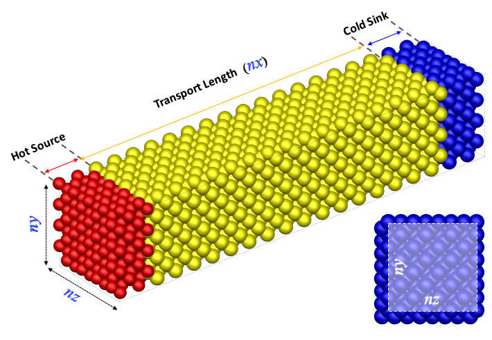
The model can be divided into three parts. 'Hot Source' to which heat is applied, 'Transport Length' to which the heat is moved, and 'Cold Sink' to which is a low-temperature region. The unit cell of both ends fixes to consider as the suspended region of experiment. The inner each 20 unit cells from the fixed range is assigned as 'Hot Source' and 'Cold Sink' by applying another temperature. The 'Transport Length' is residual subtract the 42 unit cell length to total length.
After the job has finished, click 'Update' button to update the job status. Then you can see the results at the 'Analysis' tab.
The 'Analysis' tab of LAMMPS (Thermal Conductivity) consisted of the result data and three graphs.
'Thermal Conductivity', 'Length', and 'Cross-section' are shown.
It represents the temperature distribution of the hot, transport and cold region.
It shows the change of the heat flux per unit volume and time.
It shows the cumulative energy with respect to simulation time.
Thermal conductivity simulation needs a massive model. So the model is made in the LAMMPS (Thermal Conductivity) module by determining the model size, instead of modeling that directly in the structure builder module. Therefore, connect the module to the structure builder module, which modeled the orthogonal unit cell, to perform thermal conductivity simulation with LAMMPS (Thermal Conductivity) module.
Following is the model used for the simulation.
The model can be divided into three parts. 'Hot Source' to which heat is applied, 'Transport Length' to which the heat is moved, and 'Cold Sink' to which is a low-temperature region. The unit cell of both ends fixes to consider as the suspended region of experiment. The inner each 20 unit cells from the fixed range is assigned as 'Hot Source' and 'Cold Sink' by applying another temperature. The 'Transport Length' is residual subtract the 42 unit cell length to total length.
- Select the appropriate forcefield for the system.
- Set the direction of the axis where the heat transfer will occur.
- Determine the size of the simulation model.
- Set the desired temperature of the system. (ΔT = 30 K)
- Determine the total simulation time.
- Specify the interval between each time step in the simulation.
- Set a job name and click 'Start Job!' button to start the calculation.
After the job has finished, click 'Update' button to update the job status. Then you can see the results at the 'Analysis' tab.
The 'Analysis' tab of LAMMPS (Thermal Conductivity) consisted of the result data and three graphs.
'Thermal Conductivity', 'Length', and 'Cross-section' are shown.
It represents the temperature distribution of the hot, transport and cold region.
It shows the change of the heat flux per unit volume and time.
It shows the cumulative energy with respect to simulation time.
This is the exclusive module for evaluating the plasticity and the motion of dislocations. "Dislocation" module enables to calculate the critical resolved shear stress and to evaluate the mobility of a dislocation. You may get the stress-strain curve and the structure variations during shear deformation.
Dislocation shear simulation needs a massive model. So the model is made in the LAMMPS (Dislocation Shear Simulation) module by determining the model size, instead of modeling that directly in the structure builder module. Therefore, connect the module to the structure builder module, which modeled the orthogonal unit cell, to perform the dislocation shear simulation with LAMMPS (Dislocation Shear Simulation) module.
Following is the model used for the simulation.
Models should be chosen between edge dislocation and screw dislocation. Both two models can be commonly divided into two parts. 'Fixed layer’ to which stress is applied, and 'Deformation region’ to which is deformed by the applied stress. 'Fixed layer’ is fixed to consider as the suspended region of experiment. This region is set to a length equal to 10 times of the first nearest distance from the unitcell in the structure builder module. This is kept in mind when using this module.
After the job has finished, click 'Update' button to update the job status. Then you can see the results at the 'Analysis' tab. The 'Analysis' tab of LAMMPS (Dislocation) consisted of the result data and a graph.
It represents to analyze the type of crystal structure of simulated sample.
It shows to analyze the burgers vector and line length of a dislocation.
It shows the shear stress with respect to the shear strain.
Dislocation shear simulation needs a massive model. So the model is made in the LAMMPS (Dislocation Shear Simulation) module by determining the model size, instead of modeling that directly in the structure builder module. Therefore, connect the module to the structure builder module, which modeled the orthogonal unit cell, to perform the dislocation shear simulation with LAMMPS (Dislocation Shear Simulation) module.
Following is the model used for the simulation.
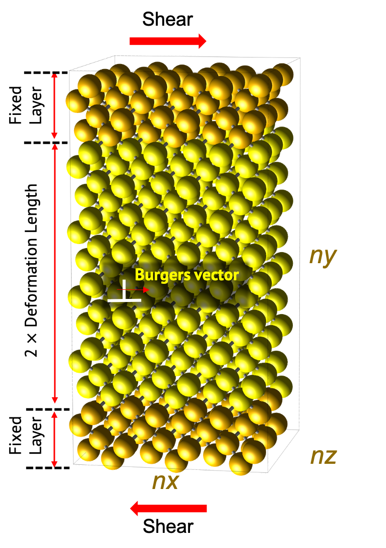 | 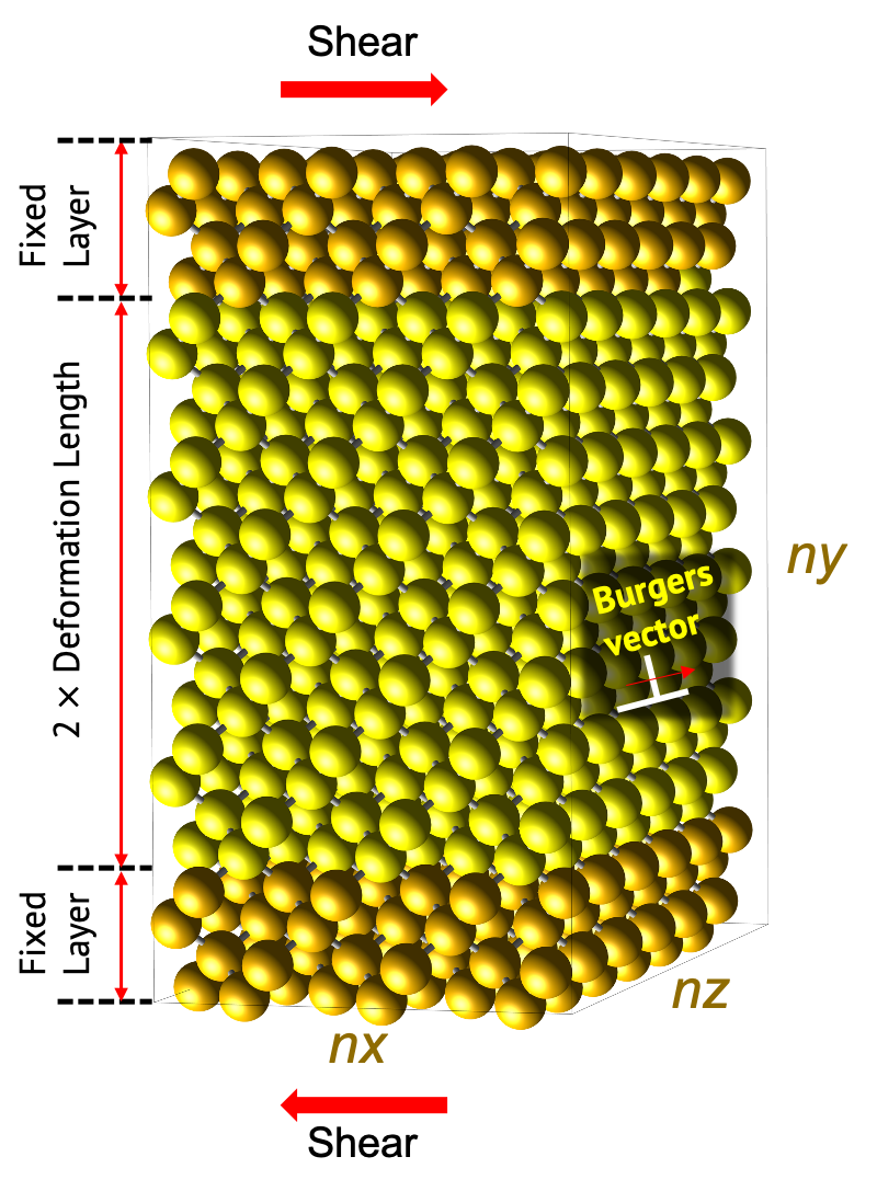 |
Models should be chosen between edge dislocation and screw dislocation. Both two models can be commonly divided into two parts. 'Fixed layer’ to which stress is applied, and 'Deformation region’ to which is deformed by the applied stress. 'Fixed layer’ is fixed to consider as the suspended region of experiment. This region is set to a length equal to 10 times of the first nearest distance from the unitcell in the structure builder module. This is kept in mind when using this module.
-
FCC <110>{111} slip system : →
 → Select FCC (111)
-
BCC <111>{110} slip system : → → Select BCC (110)
- Select the appropriate interatomic potential for the system.
- Select the type of crystal structure of unit cell. (FCC or BCC)
- Determine the size of the simulation model.
- Select the kind of dislocations. (Edge or Screw)
- Set the proper Poisson`s ratio (the metal is normally 0.3).
- Determine the displacement to shear direction.
- Set the total shear strain.
- Normal direction and glide direction of the dislocation should be moderately long to estimate more accurate results.
- In the case of the edge dislocation shear simulation, the Z size of the supercell should be at least three times of the unit cell in the z direction.
- In the case of the screw dislocation shear simulation, the both X and Z size of the supercell should be moderately long to estimate more accurate results.
- Please note that a lot of charges may be added if the supercell is too large.
- The calculation times are fast but can be inaccurate if the displacement is too large. Meanwhile, the calculation times are too slow if the displacement is too small.
- If the total shear strain is small, only the elastic region is calculated. Therefore, the proper total shear strain should be given.
After the job has finished, click 'Update' button to update the job status. Then you can see the results at the 'Analysis' tab. The 'Analysis' tab of LAMMPS (Dislocation) consisted of the result data and a graph.
It represents to analyze the type of crystal structure of simulated sample.
It shows to analyze the burgers vector and line length of a dislocation.
It shows the shear stress with respect to the shear strain.
"Tensile" module is the template for the tensile test simulation. You can simulate the tensile strength for the system by a few clicks. Select the template and connect to the structure builder which modeled the unit cell.
Cascade simulation needs massive model. So the model is made in the LAMMPS (CAS) module by determining the model size, instead of modeling that directly in the structure builder module. Therefore, connect the module to the structure builder module which modeled the unit cell to perform cascade simulation with LAMMPS (CAS) module.
After the job has finished, click 'Update' button to update the job status. Then you can see the results at the 'Analysis' tab.
In this tab, you can find the Young' modulus, Ultimate Tensile Strength (GPa), the trajectory movie, and the stress-strain curve. The Young's Modulus and Ultimate Tensile Strength is the estimation for the general stress-strain curve, so it may have some difference for the real value.
Cascade simulation needs massive model. So the model is made in the LAMMPS (CAS) module by determining the model size, instead of modeling that directly in the structure builder module. Therefore, connect the module to the structure builder module which modeled the unit cell to perform cascade simulation with LAMMPS (CAS) module.
- Select the appropriate forcefield for the system.
- Select the direction to measure the tensile strength.
- Determine the size of the simulation model. It duplicates the model of the structure builder to make a supercell.
- Write the simulation temperature.
- Determine the scale of the structural deformation. (1. Constant strain rate (ps-1), 2. Constant speed (Å/ps))
N.B. The total strain rate can calculate by 'Strain rate (ps-1) * Time (ps)'. - Set the total simulation time.
- Determine the interval to perfrom time integration (timestep).
- Set a job name and click 'Start Job!' button to start the calculation.
After the job has finished, click 'Update' button to update the job status. Then you can see the results at the 'Analysis' tab.
In this tab, you can find the Young' modulus, Ultimate Tensile Strength (GPa), the trajectory movie, and the stress-strain curve. The Young's Modulus and Ultimate Tensile Strength is the estimation for the general stress-strain curve, so it may have some difference for the real value.
“Melting and Quenching” module is able to abruptly increase (melt) or decrease (quenching) temperature to the system. Generally, this module can be used for amorphous structure generation at given temperature, radial distribution function (RDF), angular distribution function (ADF) and temperature profile are provided.
After the job has finished, click 'Update Status' button to update the job status. Then you can see the results at the 'Analysis' tab.
You can see the trajectory movie, Radial distribution function (RDF), Angle distribution function (ADF) and temperature profile.
- Select an appropriate forcefield for the system.
- Determine the size of the simulation model. Create a supercell by duplicating the connected structure builder model as many as the number of inputs.
- Set the starting and final temperature of the simulation.
- Determine the quenching (melting) rate.
- Set the pressure that will be applied to the system.
- Set the number of bins to determine how many segments from the cutoff radius.
- Determine the total simulation time.
- Specify the interval between each time step in the simulation.
- Set a job name and click 'Start Job!' button to start the calculation.
After the job has finished, click 'Update Status' button to update the job status. Then you can see the results at the 'Analysis' tab.
You can see the trajectory movie, Radial distribution function (RDF), Angle distribution function (ADF) and temperature profile.
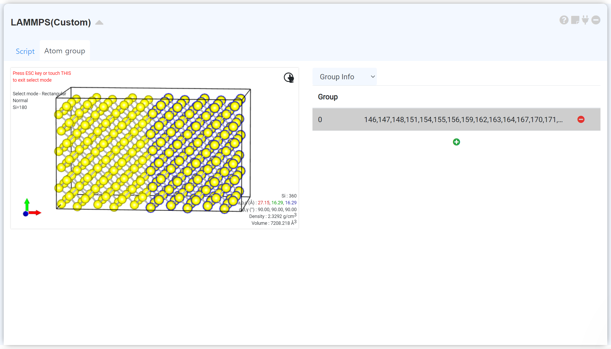
"Custom" module is for performing MD simulation which is not offered in the template. It enables perform simulation by adjusting ensemble, temperature, time. It can add options to certain atom-group by generating a group. In the present, the reactive forcefield (ReaxFF) only supported, but other types of potential will be updated soon.
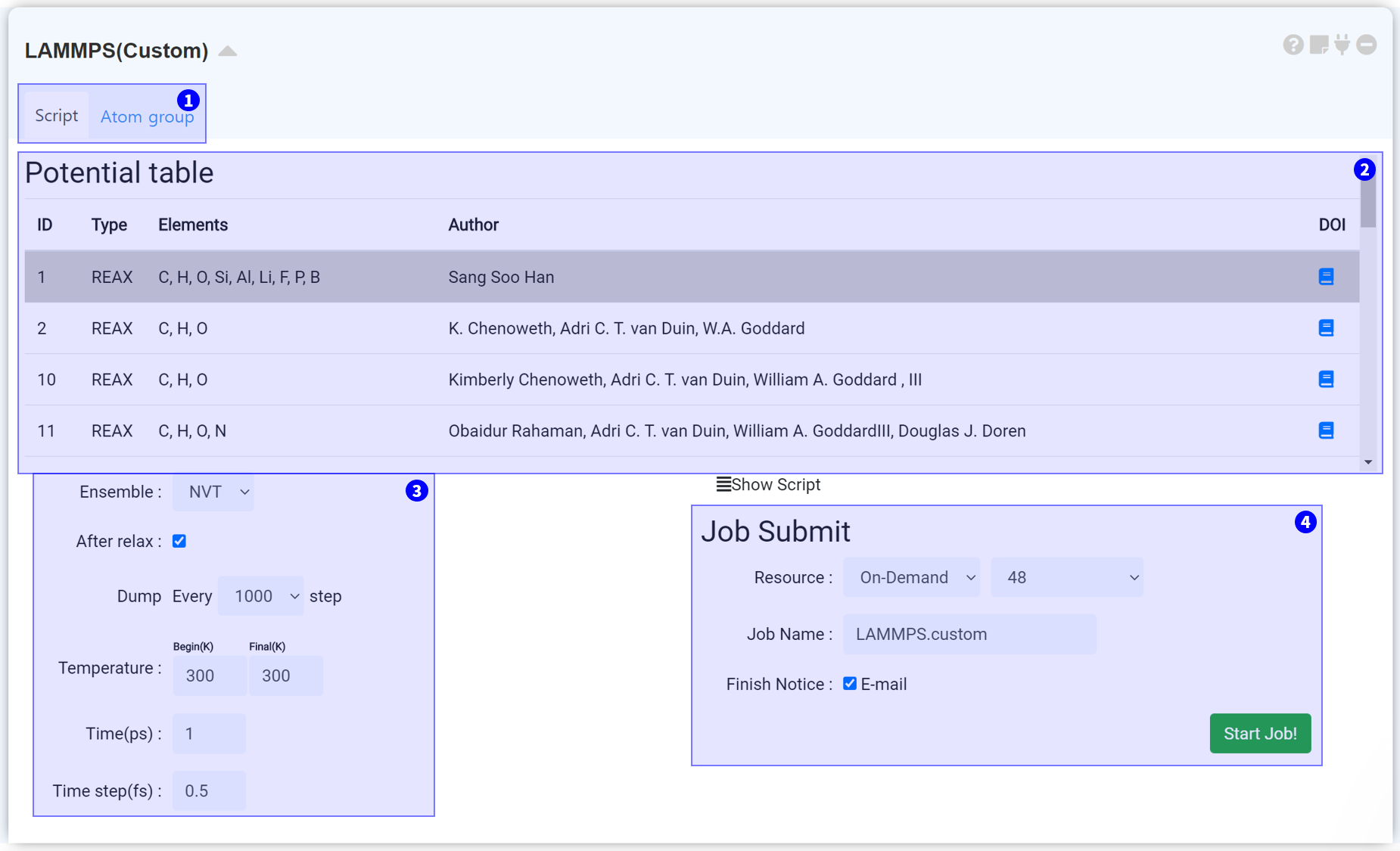
The LAMMPS module consist of two tabs. You can choose a forcefield and input parameters and submit a job to the cloud computing server to start MD simulation in the Script tab.
If you want to adjust simulation precisely by setting a specific atom group, make a new atom group and adjust the velocity, force, move, and temperature in the AtomGroup tab. Refer to the following 'Grouping' section for a detailed description.
It is a list to select a forcefield which is necessary for MD simulation. We provide a reactive forcefield as a default. We will support the other MD potentials in the future.
In this section, you can set the input parameters of LAMMPS for MD simulation. You can adjust ensemble, After Relax, Dump, Temperature, and Time. See the appendix for more information on the LAMMPS input settings.
After finishing the setting, submit the job to cloud server by referring to the Job submit section.
LAMMPS can give an initial condition to a specific atom group. Click the AtomGroup tab to display a visualizer. The visualizer contains the structure information when the module is connected to the structure builder. Activate a select menu at the right-click popup window, and select the atoms that you want to add the additional setting. If you click the +, the new atom group will be added.
You can add Atom groups as much as you want. Click a previously set Atom group on the list. It displays only the atoms belonging to that Atom group. Select the groupwhich you want to set the initial condition, and click Group Info to select the desired condition. Check the checkbox, and set the condition to be applied in each axis direction.
This module generates a "densely packed simulated polymer model" which is thermally equilibrated at a specific temperature and normal density.
Click the 'Update Status' button to update the module after finishing the calculation. Then, you can check the obtained results on the 'Analysis' tab.
You can analyze the 'Trajectory movie, Temperature, Volume, Energy' data.
- Select the appropriate potential for the system. 'Dreiding' is the default.
- Check the basic properties: Bond scale, Charge equilibrate method, Long range interaction distance, Coulombic interaction
- Click the to perform the preliminary structure optimization. It is recommended to click the to submit the optimization job to the cloud server if the system has a lot of atoms. (The molecular structure complexity can make reproduction difficult.)
- Determine the temperature of the system.
- Specify the density that the system will have.
- If you need, change the additional parameters in more detail under the Advanced Options.
- Set the job name.
- Click the 'Start Job!' button to start the calculation.
Click the 'Update Status' button to update the module after finishing the calculation. Then, you can check the obtained results on the 'Analysis' tab.
You can analyze the 'Trajectory movie, Temperature, Volume, Energy' data.
"LAMMPS (Tg/CTE)" module is for calculating the Glass transition temperature and Constant of thermal expansion (CTE) of a polymer system.
This module is the "Restart" module that should be performed following thermalization. Add this module, and connect with the successfully finished LAMMPS (Thermalization) module. The forcefield is automatically set from the connected thermalization module.
Click the 'Update Status' button to update the module after finishing the calculation. Then, you can check the obtained results on the 'Analysis' tab.
Here, you can analyze the 'Trajectory movie', 'Volume vs Temperature', 'CTE vs Volume', 'Temperature profile', 'MSD' data.
This module is the "Restart" module that should be performed following thermalization. Add this module, and connect with the successfully finished LAMMPS (Thermalization) module. The forcefield is automatically set from the connected thermalization module.
- Set the precision of the calculation. This option affects the number of data. In other words, it determines the temperature interval between data.
- Determine the initial and final temperature of the system.
- If you need, change the additional parameters in more detail under the Advanced Options.
- Set the job name.
- Click the 'Start Job!' button to start the calculation.
Click the 'Update Status' button to update the module after finishing the calculation. Then, you can check the obtained results on the 'Analysis' tab.
Here, you can analyze the 'Trajectory movie', 'Volume vs Temperature', 'CTE vs Volume', 'Temperature profile', 'MSD' data.
"LAMMPS (Elastic properties)" module is for calculating the elastic property of a polymer system.
This module is the "Restart" module that should be performed following a glass transition temperature calculation. Add this module, and connect with the successfully finished LAMMPS (Tg/CTE) module. The forcefield is automatically set from the connected LAMMPS (Tg/CTE) module.
Click the 'Update Status' button to update the module after finishing the calculation. Then, you can check the obtained results on the 'Analysis' tab.
Here, you can see the 'Bulk modulus', 'Shear modulus', 'Young's modulus', 'Poisson's ratio' data.
This module is the "Restart" module that should be performed following a glass transition temperature calculation. Add this module, and connect with the successfully finished LAMMPS (Tg/CTE) module. The forcefield is automatically set from the connected LAMMPS (Tg/CTE) module.
- Check the brought precision of the calculation and initial, final temperature of the system.
- If you need, change the additional parameters in more detail under the Advanced Options.
- Set the job name.
- Click the 'Start Job!' button to start the calculation.
Click the 'Update Status' button to update the module after finishing the calculation. Then, you can check the obtained results on the 'Analysis' tab.
Here, you can see the 'Bulk modulus', 'Shear modulus', 'Young's modulus', 'Poisson's ratio' data.
"LAMMPS (Dielectric constant)" module is for finding the electrical property of a polymer system.
This module is the "Restart" module that should be performed following thermalization. Add this module, and connect with the successfully finished LAMMPS (Thermalization) module. The forcefield is automatically set from the connected thermalization module.
It is recommended to turn on the 'Coulombic interaction' option when performing a thermalization calculation.
Click the 'Update Status' button to update the module after finishing the calculation. Then, you can check the obtained results on the 'Analysis' tab.
Here, you can find the dielectric constants as a function of the temperature.
This module is the "Restart" module that should be performed following thermalization. Add this module, and connect with the successfully finished LAMMPS (Thermalization) module. The forcefield is automatically set from the connected thermalization module.
It is recommended to turn on the 'Coulombic interaction' option when performing a thermalization calculation.
- Set the precision of the calculation. This option affects the number of data. In other words, it determines the temperature interval between data.
- Determine the initial and final temperature of the system.
- If you need, change the additional parameters in more detail under the Advanced Options.
- Set the job name.
- Click the 'Start Job!' button to start the calculation.
Click the 'Update Status' button to update the module after finishing the calculation. Then, you can check the obtained results on the 'Analysis' tab.
Here, you can find the dielectric constants as a function of the temperature.
"LAMMPS (Solubility parameter)" is for obtaining the Hildebrand Solubility Parameter of a polymer system.
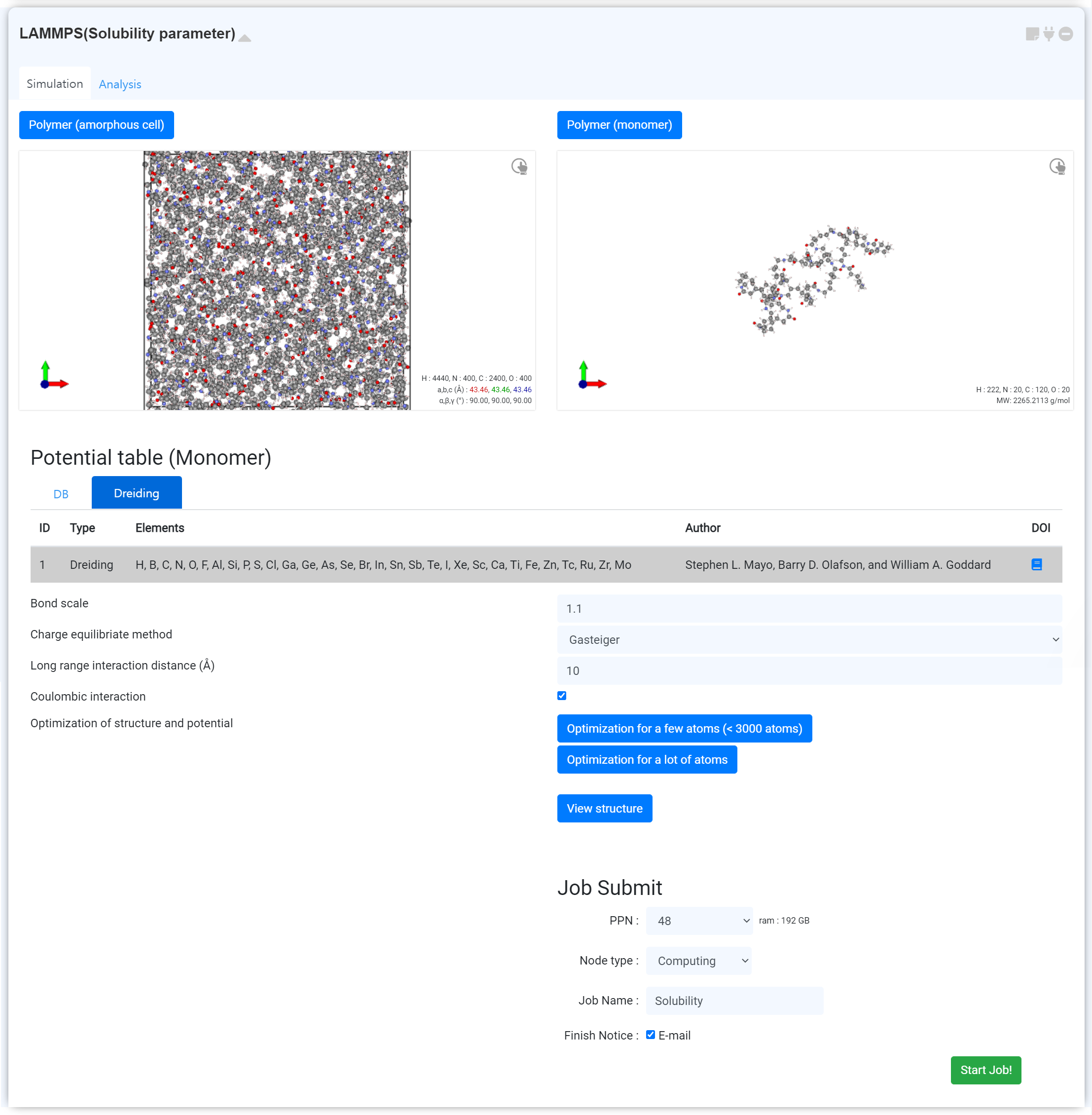
An amorphous cell and a monomer structure are required to calculate the solubility. You can import the structures from connecting with previous modules.
It is recommended to bring a polymer cell in the liquid area as the amorphous cell.
Next, set the job name and click the 'Start Job!' button to start the calculation.
The calculation will not normally proceed if you upload the structure file directly to the visualizer.
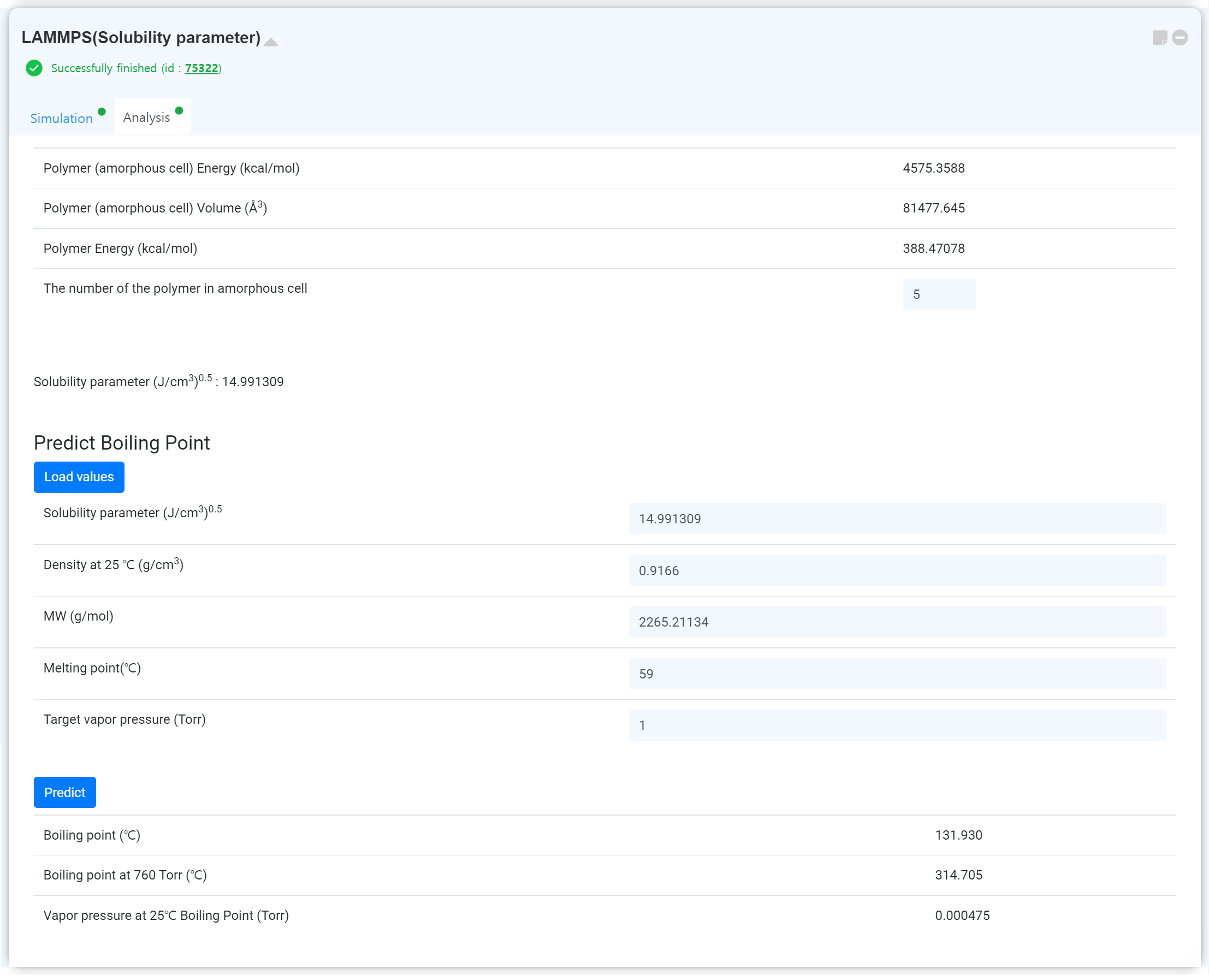
Click the 'Update Status' button to update the module after finishing the calculation. Then, you can check the obtained results on the 'Analysis' tab.
Also, you can determine the solubility parameter by changing 'The number of the polymer in amorphous cell' value.
And you can predict the boiling point from machine learning. Click the to import the calculation data. Next, click .
An amorphous cell and a monomer structure are required to calculate the solubility. You can import the structures from connecting with previous modules.
It is recommended to bring a polymer cell in the liquid area as the amorphous cell.
- LAMMPS (Thermalization)
- LAMMPS (Tg/CTE)
- Structure Builder
- Molecule Builder
Next, set the job name and click the 'Start Job!' button to start the calculation.
The calculation will not normally proceed if you upload the structure file directly to the visualizer.
Click the 'Update Status' button to update the module after finishing the calculation. Then, you can check the obtained results on the 'Analysis' tab.
Also, you can determine the solubility parameter by changing 'The number of the polymer in amorphous cell' value.
And you can predict the boiling point from machine learning. Click the to import the calculation data. Next, click .
"LAMMPS (Viscosity EMD)" module is for calculating the viscosity of the polymer structure through an equilibrium molecular dynamics simulation. This module allows you to calculate the average viscosity of the material.
This module is the "Restart" module that should be performed following thermalization. Add this module, and connect with the successfully finished LAMMPS (Thermalization) module. The forcefield is automatically set from the connected thermalization module.
It is recommended to turn on the 'Coulombic interaction' option when performing a thermalization calculation.
Click the 'Update Status' button to update the module after finishing the calculation. Then, you can check the obtained results on the 'Analysis' tab.
Here, you can check the viscosity change over time at each temperature.
This module is the "Restart" module that should be performed following thermalization. Add this module, and connect with the successfully finished LAMMPS (Thermalization) module. The forcefield is automatically set from the connected thermalization module.
It is recommended to turn on the 'Coulombic interaction' option when performing a thermalization calculation.
- Set the precision of the calculation. This option affects the number of data. In other words, it determines the temperature interval between data.
- Determine the initial and final temperature of the system.
- If you need, change the additional parameters in more detail under the Advanced Options.
- Set the job name.
- Click the 'Start Job!' button to start the calculation.
Click the 'Update Status' button to update the module after finishing the calculation. Then, you can check the obtained results on the 'Analysis' tab.
Here, you can check the viscosity change over time at each temperature.
"LAMMPS (Viscosity NEMD)" module is for calculating the viscosity of the polymer structure through a non-equilibrium molecular dynamics simulation.
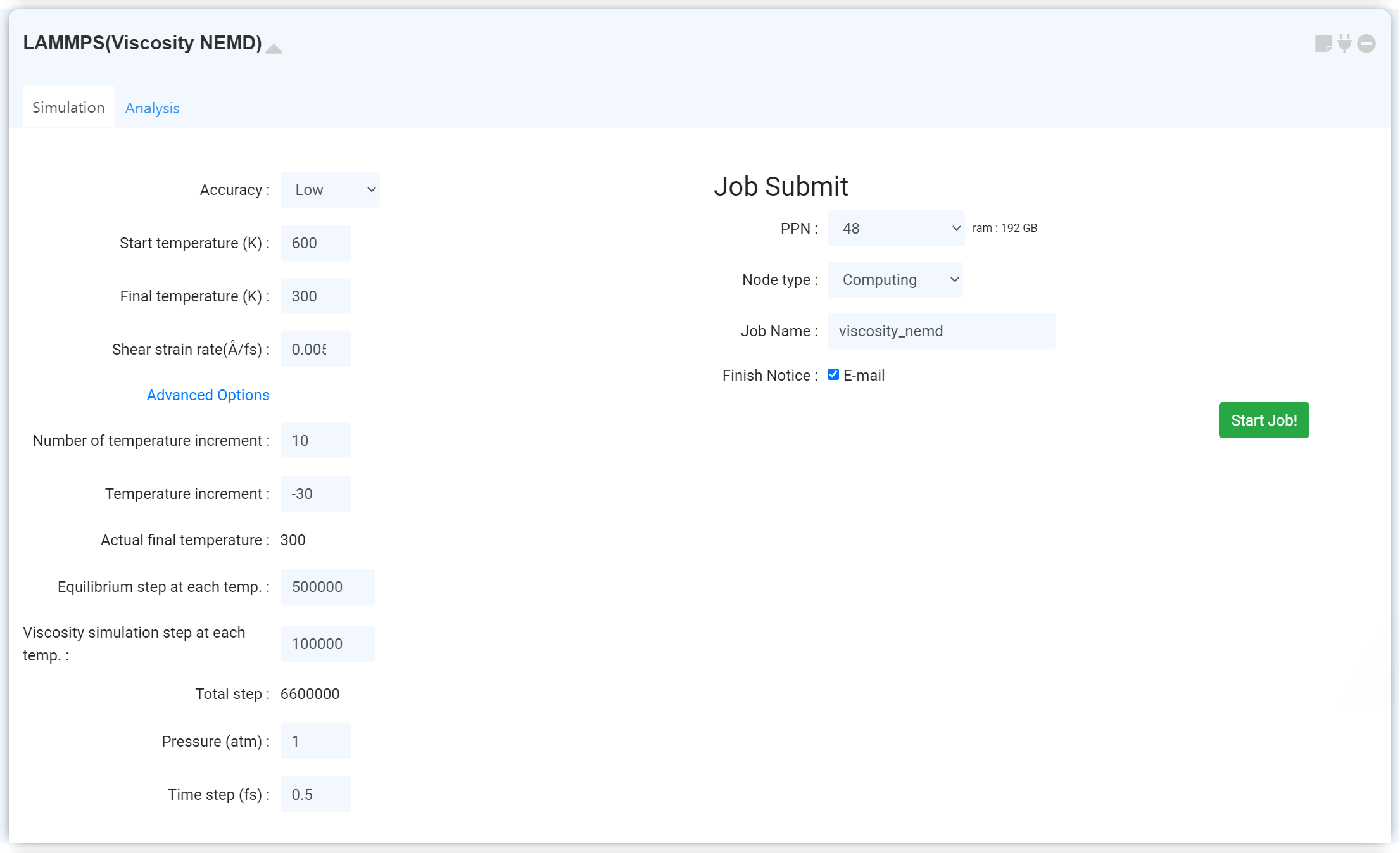
This module is the "Restart" module that should be performed following thermalization. Add this module, and connect with the successfully finished LAMMPS (Thermalization) module. The forcefield is automatically set from the connected thermalization module.
It is recommended to turn on the 'Coulombic interaction' option when performing a thermalization calculation.
Click the 'Update Status' button to update the module after finishing the calculation. Then, you can check the obtained results on the 'Analysis' tab.
Here, you can check the viscosity change over time at each temperature.
This module is the "Restart" module that should be performed following thermalization. Add this module, and connect with the successfully finished LAMMPS (Thermalization) module. The forcefield is automatically set from the connected thermalization module.
It is recommended to turn on the 'Coulombic interaction' option when performing a thermalization calculation.
- Set the precision of the calculation. This option affects the number of data. In other words, it determines the temperature interval between data.
- Determine the initial and final temperature of the system.
- If you need, change the additional parameters in more detail under the Advanced Options.
- Set the job name.
- Click the 'Start Job!' button to start the calculation.
Click the 'Update Status' button to update the module after finishing the calculation. Then, you can check the obtained results on the 'Analysis' tab.
Here, you can check the viscosity change over time at each temperature.
Calphad is the module calculating thermodynamic information of various materials. Refer to the
appendix
to access the detailed description and database information, examples.
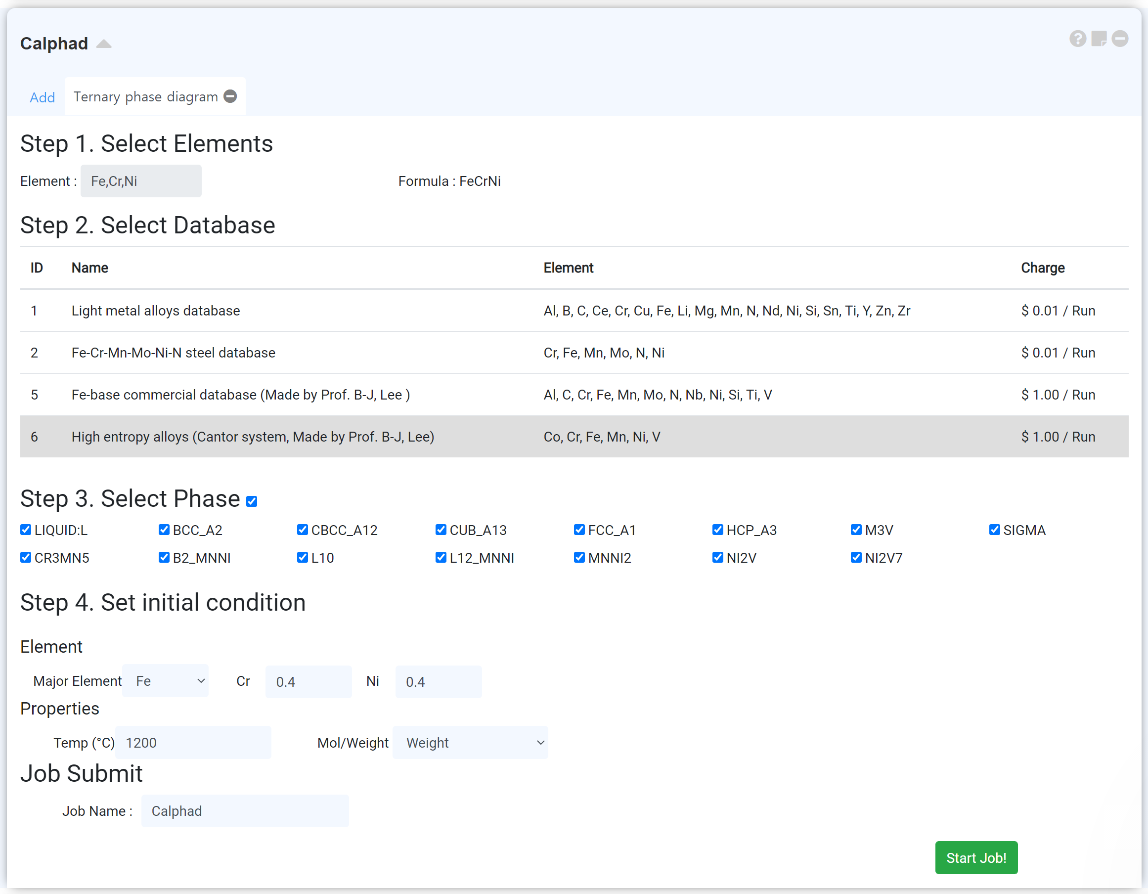
-
Select atoms what contained at the system you want to plot phase diagram. In the case of the binary, ternary phase diagram, if the element selected enough, then the periodic table closed automatically. -
Select the database which is the most appropriate for the system. Refer to the appendix to read the detailed information of the database. -
Select the phase that you want to contain when plotting the phase diagram. -
Specify the initial starting point at which the phase diagram will be plotted. If the starting point is not proper, the graph may not be drawn properly or the calculation fail.
Crystal Graph Convolutional Neural Network (CGCNN) is the most successful prediction model for the materials science field combined with the machine learning approach. You may predict the various material properties, such as formation energy, bandgap, bulk/shear moduli, Poisson’s ratio, etc., through the material structure as an input.
You can upload and check the training dataset in “Check Dataset” tab. Click the Upload zip file button to upload the database zip file.
1) “Zip file” consists of two parts, structure files (cif format) and property files (id_prop.csv).
2) “id_props.csv” should includes structure name (1st column, e.g. mp-100, mp-101, mp-102 …) and desired property (2nd column, e.g. 1.13, 1.42, 2.43, 1.22 …) value.
This part is for making your own machine-learning model. You can design your own machine learning model, from how to make the machine learning model by determining how to distribute the learning data and test data, to adjusting various hyper-parameters, and the optimizing method for learning. It consists of Dataset ratio, Layers, related to the network, Other options, related to optimizing.
After finishing the setting, submit the job by referring Job submit section.
After finishing the calculation, “CGCNN Result” tab shows the accuracy of the your own CGCNN model.
You can check the value of loss function with the learning/test data as a function of epoch. Generally, the accuracy of the learning data is higher than the test data. But if the accuracy of the learning data is too high, you should consider overfitting issue.
After finishing the learning, “CGCNN Predict” tab enables loading the calculated module to predict the properties of uploaded other structures. Click the Upload zip file button to upload the database zip file.
“Zip File” should include structure files (cif format) only.