MatSQ has modularized each function, making it easy to add and modify functions.
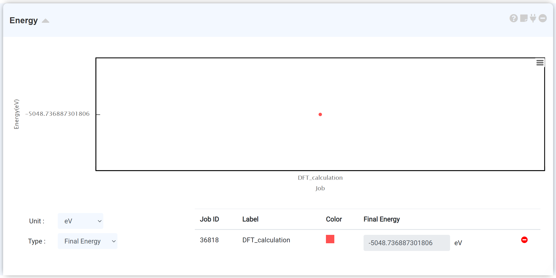
Each calculation job can consist of several scf steps, and one scf step consists of a set of iteration steps. The Energy module plots the total energy value obtained from the iterative self-consistent calculation. Therefore, for a calculation that performs a single scf calculation, there is only one data point because only one total energy data was obtained through iteration. The optimization calculation (QE: (vc-)relax, GAMESS: OPTIMIZE), which consists of several scf steps, shows the energy that gradually changing with the progress of the scf calculation.
For more information on the self-consistent calculation, refer to the Blog, official website of the Quantum Espresso or GAMESS.
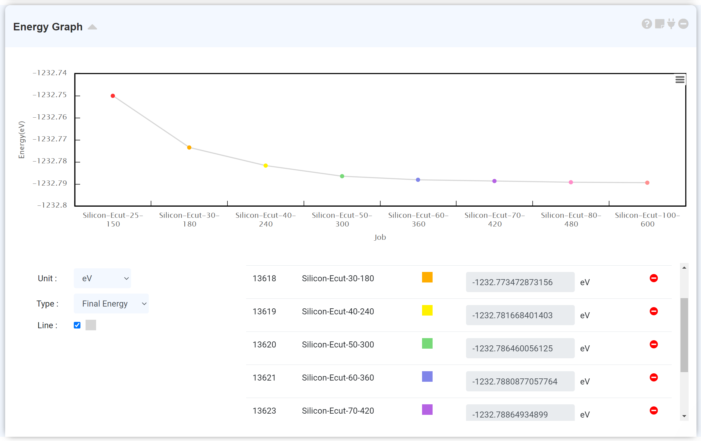
Checking the energy graph is a good way to ensure that convergence has been achieved during the structural optimization process. The calculation may not have been completed properly if the scf phase of the energy graph has reached the maximum number of scf steps even if the “This job is normal finished” message appeared in the QE module. Refer to the Restart job (Quantum Espresso) , Restart job (GAMESS) section.
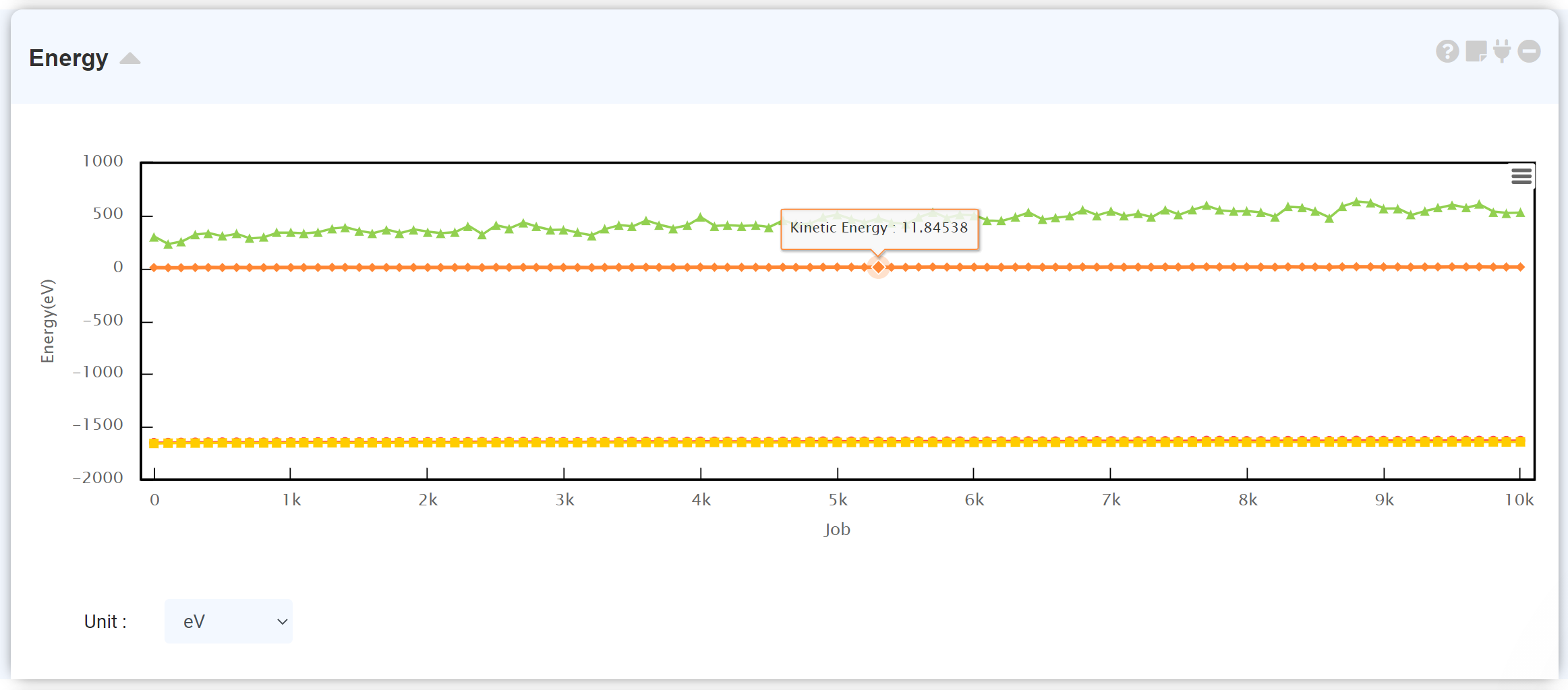
Connect the energy module to the calculation finished LAMMPS module to see the energy change during the MD simulation.
At the setting window, set the time and step to next trajectory. At input area of Move, put desired step and click Move button, you can see the trajectory and data at that step.
Use the Compare Structure module to compare two structures at a glance.
This module can be linked to the 'Structure Builder', 'Quantum Espresso', and 'LAMMPS (Custom) modules which having a structural information. After adding this module, connect it to the module desire to compare and assign the structure to the 'Structure A.'
Connecting to the Simulation module allows you to choose the 'initial' or 'final' structure.
When performing a structural optimization with (vc-)relax, which finds the local minimum from the potential energy curve of the system at the Quantum Espresso module, it is recommended to compare the initial and final structures to check the structural changes in the relaxation process.
When you connect this module to the LAMMPS (Custom) module, you can compare the initial (step 0) and final (last step) structures.
Alternatively, you can place two different structures side by side to see the difference.
The Compare Structure module consists of two visualizer canvases and a data table. Selecting the “Sync” checkbox synchronizes the time points. If you place the cursor over the table, the corresponding atom shows in lignt-brown. The movement of atoms in the table is indicated by an orthogonal coordinate (Å).
Enter several data to draw trend line.
'Custom' option enables write your custom equation. Please refer to the following cautions.
- Write the number of the coefficient exactly at the '# Coeffs. (Number of Coefficients)' input window.
- Do not omit the multiplication sign '*' when entering the equation to 'Equation' input window.
- Do not write 'y=' when entering the equation to the 'Equation' input window.
- You can use only a, b, c, d, e, f symbol for the coefficients when entering the equation to the 'Equation' input window.
This module is for checking basic calculation results and NMR data after DFT calculation using the Quantum Espresso module.
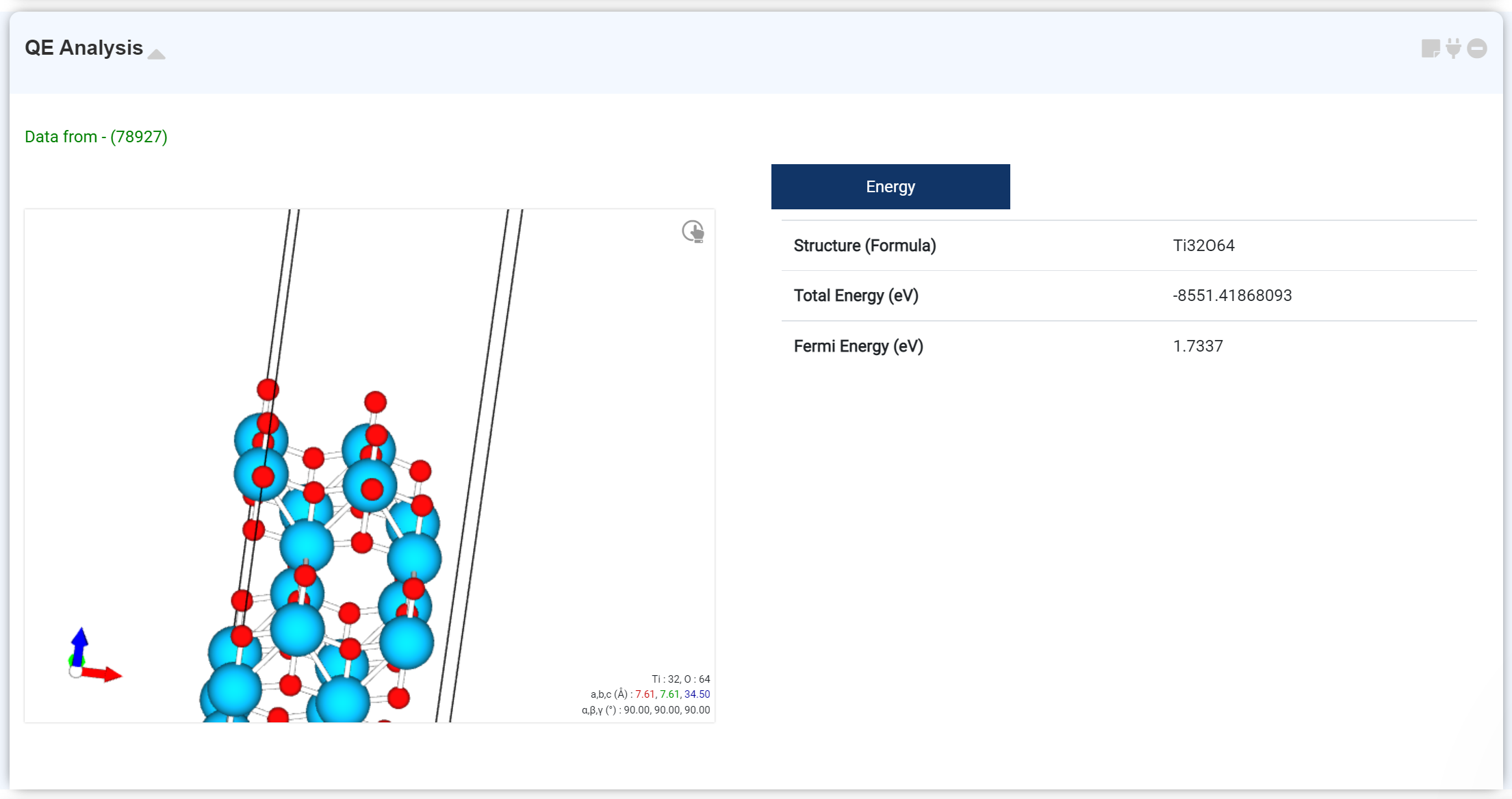
You can check the basic calculation results on this tab. The checkable information is:
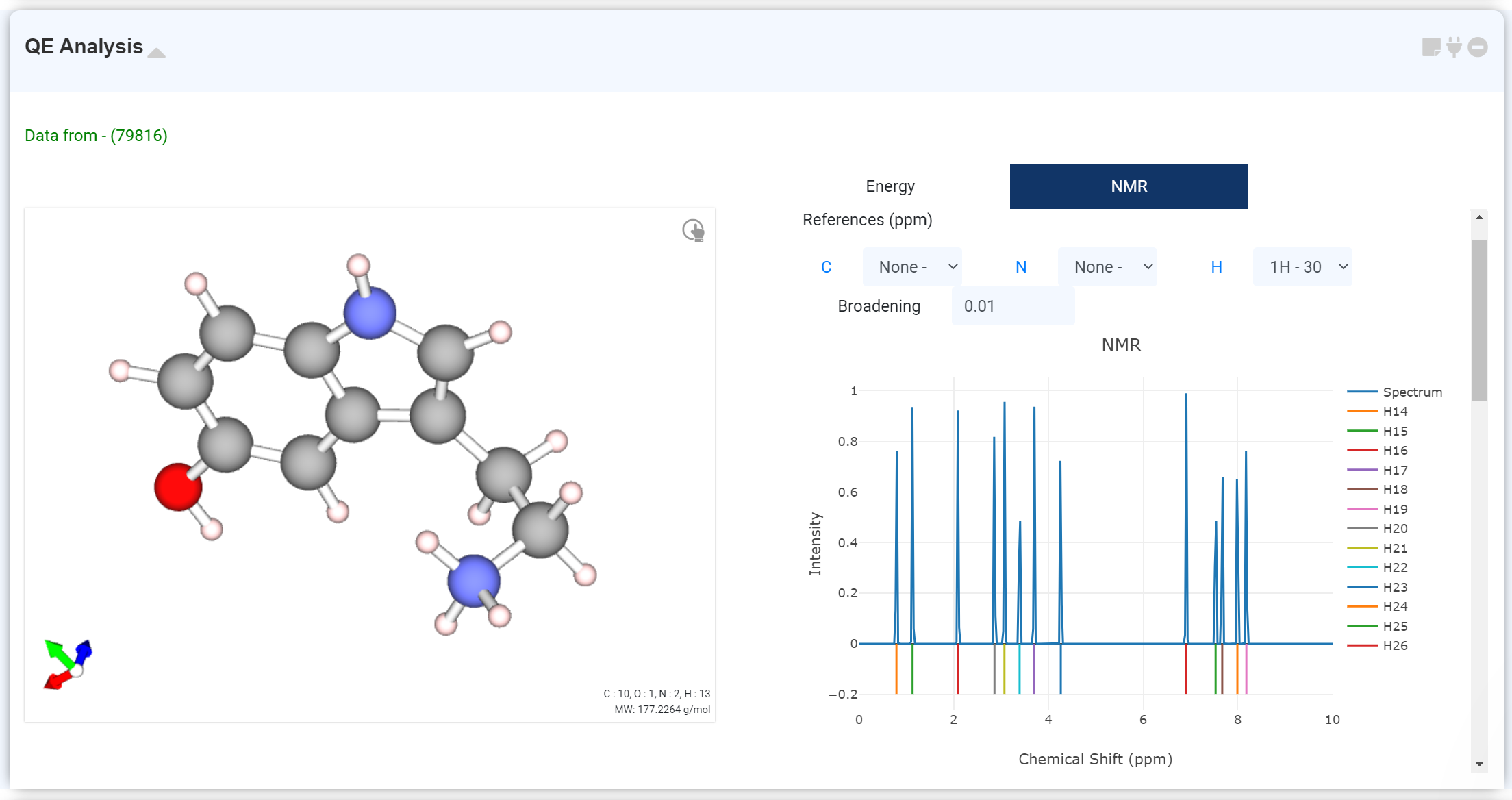
You can check the NMR calculation result on this module If NMR calculation is performed by adding the NMR solver tab to the Quantum Espresso module.
Scroll down to see a table with atoms and computed NMR data. Select the desired atoms in the table to add the corresponding values to the spectrum. Alternatively, you can click the blue element symbol link next to the to see the data for that element at once. The Select box allows you to specify a reference to compensate for the x-axis (chemical shift) values. Adjust the Spectrum shape by modifying the Broadening values.
You can check the basic calculation results on this tab. The checkable information is:
- Optimized structure
- Formula
- Total Energy
- Fermi Energy
You can check the NMR calculation result on this module If NMR calculation is performed by adding the NMR solver tab to the Quantum Espresso module.
Scroll down to see a table with atoms and computed NMR data. Select the desired atoms in the table to add the corresponding values to the spectrum. Alternatively, you can click the blue element symbol link next to the to see the data for that element at once. The Select box allows you to specify a reference to compensate for the x-axis (chemical shift) values. Adjust the Spectrum shape by modifying the Broadening values.
- Charge Density Difference

- STM Image
Click on
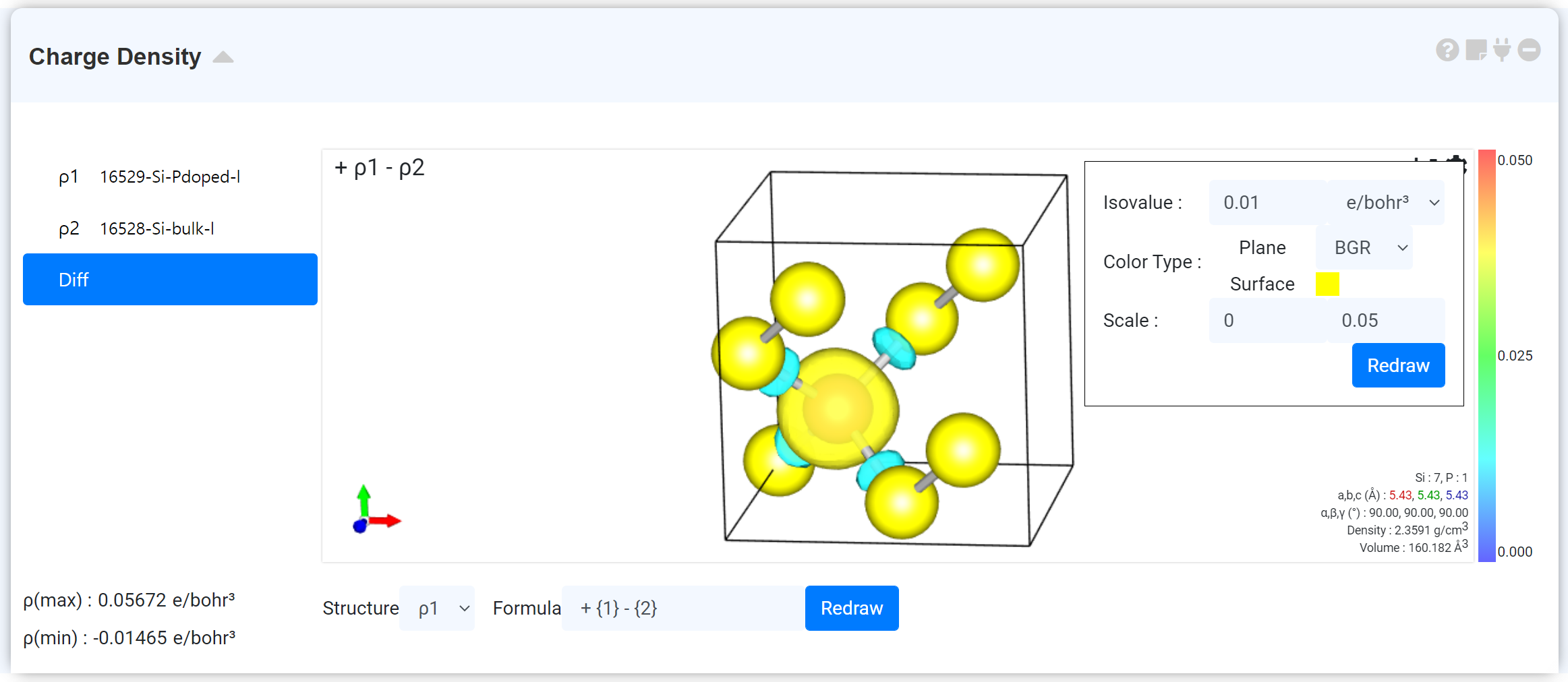
You can change the charge density-related settings by clicking on [toothed wheel] in the upper right corner of Visualizer. You can change the isovalue taking account of the ρ (max) and ρ (min) values located in the lower-left corner to change the surface or the color of the cross-section and the gradation scale value of the surface color.
If more than one charge densities are connected, 'Diff' tab is activated with the connected charge densities in the list on the left. You can view the sum or difference of the charge density values, which were connected through Diff. Refer to the following section for more information on how to draw charge density differences. Note: “charge density” refers to an electron density by convention of DFT society. This module draws ‘pseudo charge density’ which is much smoother near atomic cores than true chare density, as Quantum Espresso uses pseudopotential.
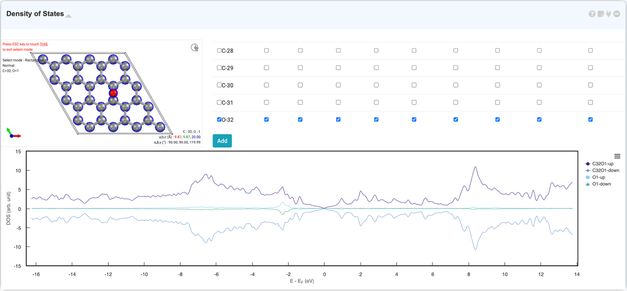
The Density of States graph shows the number of electronic states at particular eigenvalue. The DOS graph is represented by Energy (eV) vs. the number of states (#/eV).
See the graph in detail by dragging the mouse. And also, you can set the axis-range and the legend on the right-click setting window.
In 'Visualizer' of the DOS module, you can select only a specific atom and select a specific orbital from the 'Orbital list' on the right to view the PDOS (projected density of states) for that.
For example, if you want to see the surface state occurs from what chemical species, add PDOS. If you select the desired atoms in the 'Visualizer canvas', the corresponding orbitals only appear in the right of 'Orbital table'. Select desired orbitals and click the 'Add' button to add PDOS. Now you can see which orbital of what atom corresponds to this state.
DOS can be combined with a band structure diagram (refer to the Band Structure Section.) The x-axis of the DOS graph is the same as the y-axis of the band diagram. The bandgap on both graphs is the same.
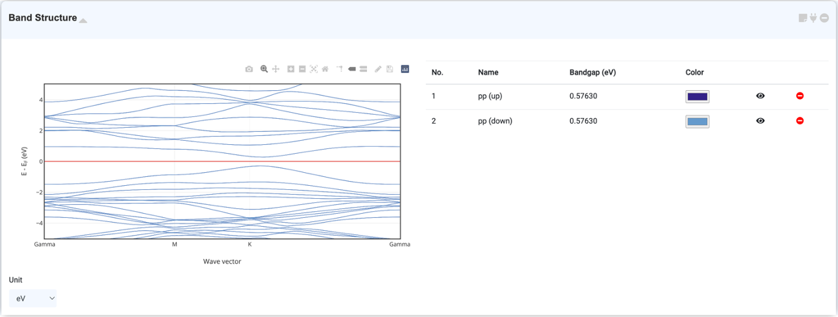
The Band Structure module is a module for drawing a band structure obtained from a band structure calculation. Refer to the Band Structure Calculation documentation for instructions on how to calculate the band structure.
Press
The x-axis of the band diagram, the k-path label, is automatically set by finding the crystal system point set that has the highest similarity among high-symmetric points. You can change the crystal system and energy units in the Select Box.
You can connect a Quantum Espresso module with DOS data to view a band structure and a DOS graph side by side. The y-axis of the band diagram is the same as the x-axis of the DOS graph. You can zoom in by dragging with the mouse and return to the original using the Reset button in the upper right corner of the graph. The table at the bottom of the graph allows you to clear or disable the chart drawn on Canvas.
You can project a band structure and DOS on the specific atom and orbital, and draw a fat band. For more information, see the following ‘Projected Band Structure’ section.
If you want to see a projected band structure on a specific atom or orbital, or if you want to draw a fatband, perform a projection calculation by adding a DOS solver to the Quantum Espresso module that calculated the band structure.
Press the
The added data is displayed in either a circle or a bold line. The sum of the contributions of the selected orbitals at that point determines the diameter of the circle or the thickness of the line. Contribution refers to the distribution of each orbital to the eigenvalue at that point. The color of the graph is the average value of the selected orbital color having the same angular momentum quantum number.
If the added data contains multiple data with different angular momentum quantum numbers, the contribution of each orbital is displayed in color gradient. If you want to view the contribution of each orbital as the radius of the circle/the thickness of the line, select each orbital separately and add it.
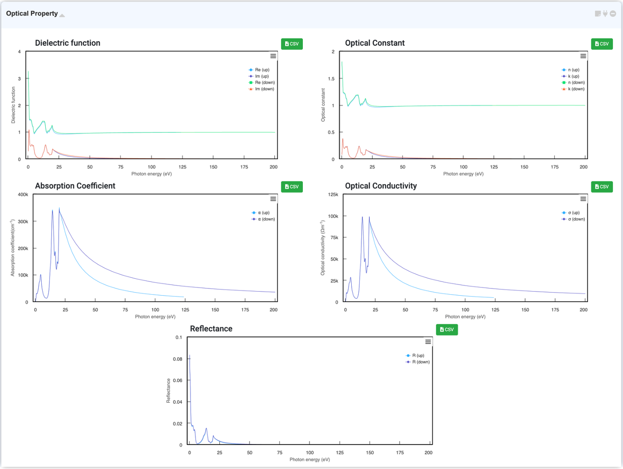
It enables to check the optical properties calculated from the 'Quantum Espresso' module. You can easily calculate various optical properties of a material based on the plane-wave basis DFT calculation. One provides the real and imaginary parts of the dielectric tensor or the joint density of states. Only supported Norm-Conserving Pseudopotential (LDA and GGA).
- Dielectric function
- Joint density of state (JDOS)
- Refractive index
- Absorption coefficient
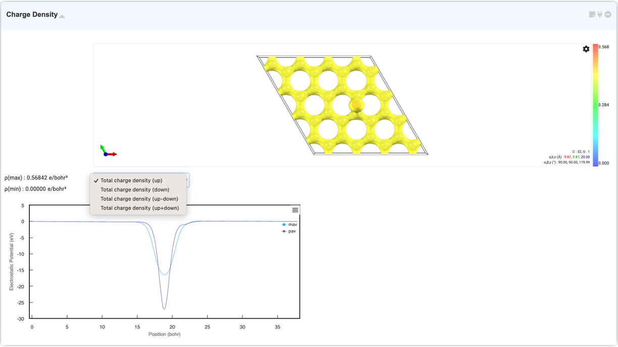
The "Charge Density" module visualizes the charge density and potential of a calculated structure by displaying surfaces (isosurfaces) and cell boundaries with equal values in space. If you select "Charge Density" in the Analysis Module and click on the activated module to connect, the charge density and potential will appear in 3D/2D format in this module. You can change charge the settings by opening the settings window through the gear button at the top right corner of the Visualizer.
Density of state graphs provide information about the number of states occupied at a particular eigenvalue, and the graph is expressed as Energy (eV) versus the number of states (arbitrary units). You can check the DOS graph by selecting "Density of States" in the Analysis Module and clicking on the activated module to connect. You can zoom in by dragging to check the graph in detail, and you can set the axis range and legend in the right-click settings window.
The DOS module allows you to view the projected density of states (PDOS) for specific atomic orbitals. When you select the desired atom in the visualizer in the DOS module, the orbitals of the atoms are displayed in the orbital list on the right. If you select the desired orbital and click the 'Add' button, 'PDOS' will be added.
Band structure represents the energy level, or distribution, allowed for electrons in a material. The graph is represented by k vector vs energy. You can check the band structure by selecting "Band Structure" in the Analysis Module and clicking on the activated module to connect. You can zoom in, set range, download, etc. using the tools at the top.
By selecting "Optical Property" in the Analysis Module and clicking on the activated module to connect, you can check the optical properties of the system graphically. You can check Dielectric function, Optical Constant (refractive index, extinction coefficient), Absorption coefficient, Optical conductivity, and Reflectance in this module.
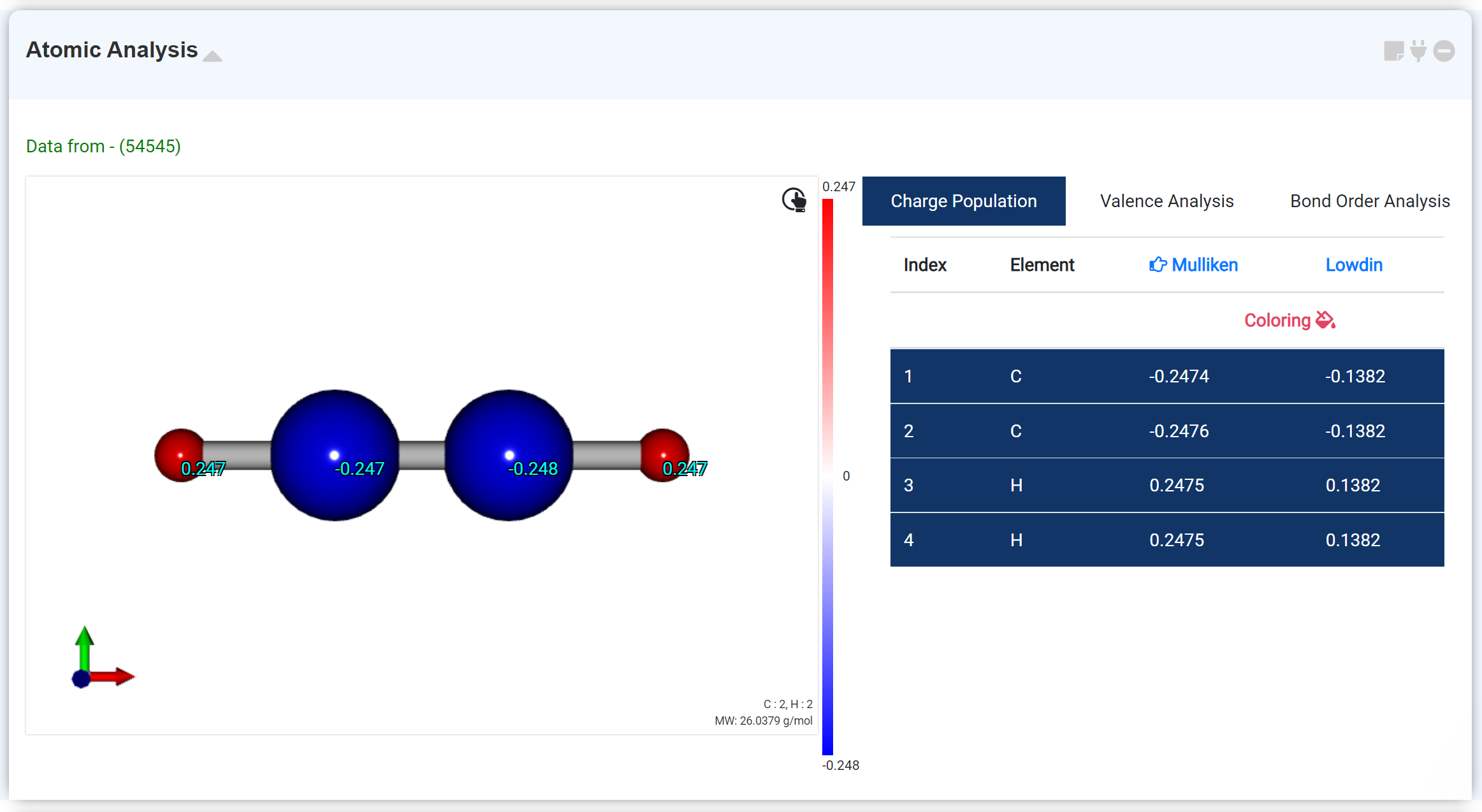
The Atomic Analysis module for analyze the calculation results obtained after geometry optimization. This moudle shows the molecule geometry, charge information, bond order.
Charge Population tab shows Mulliken and Lowdin Charge. If clicking the 'Coloring ' option, the charge transfer distribution is expressed in color.
When you click an atom in the list of the right window, the atom's information overlaps on the corresponding atom of the molecular structure of the left window. The selected charge type is marked with a finger arrow ('Mulliken' in the figure above), and users can change the type in the header section to display the desired information..
The Valence Analysis tab expresses the total valence charge and bonded valence data obtained from optimization.
The bond order of each atomic bond is indicated in the Bond Order Analysis tab.
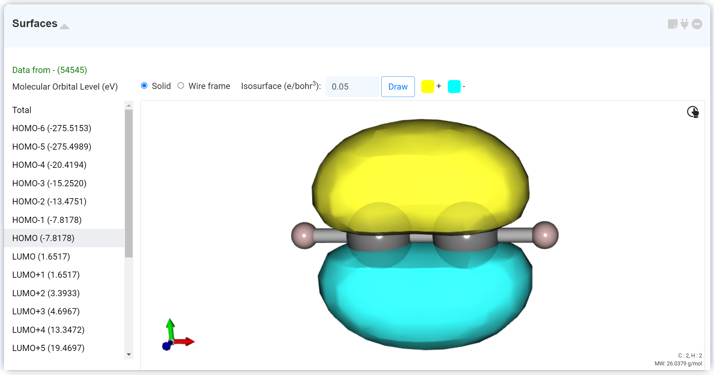
The 'Surface' module represents the calculated molecular orbital (MO) with HOMO as the default.
At the top, users can change the display format to Wireframe and adjust the Isosurface value. If an open shell calculation is performed, users can select alpha or beta spin.
The left list shows the MO eigenvalues, and each data connects to the graph in the Density of States module.
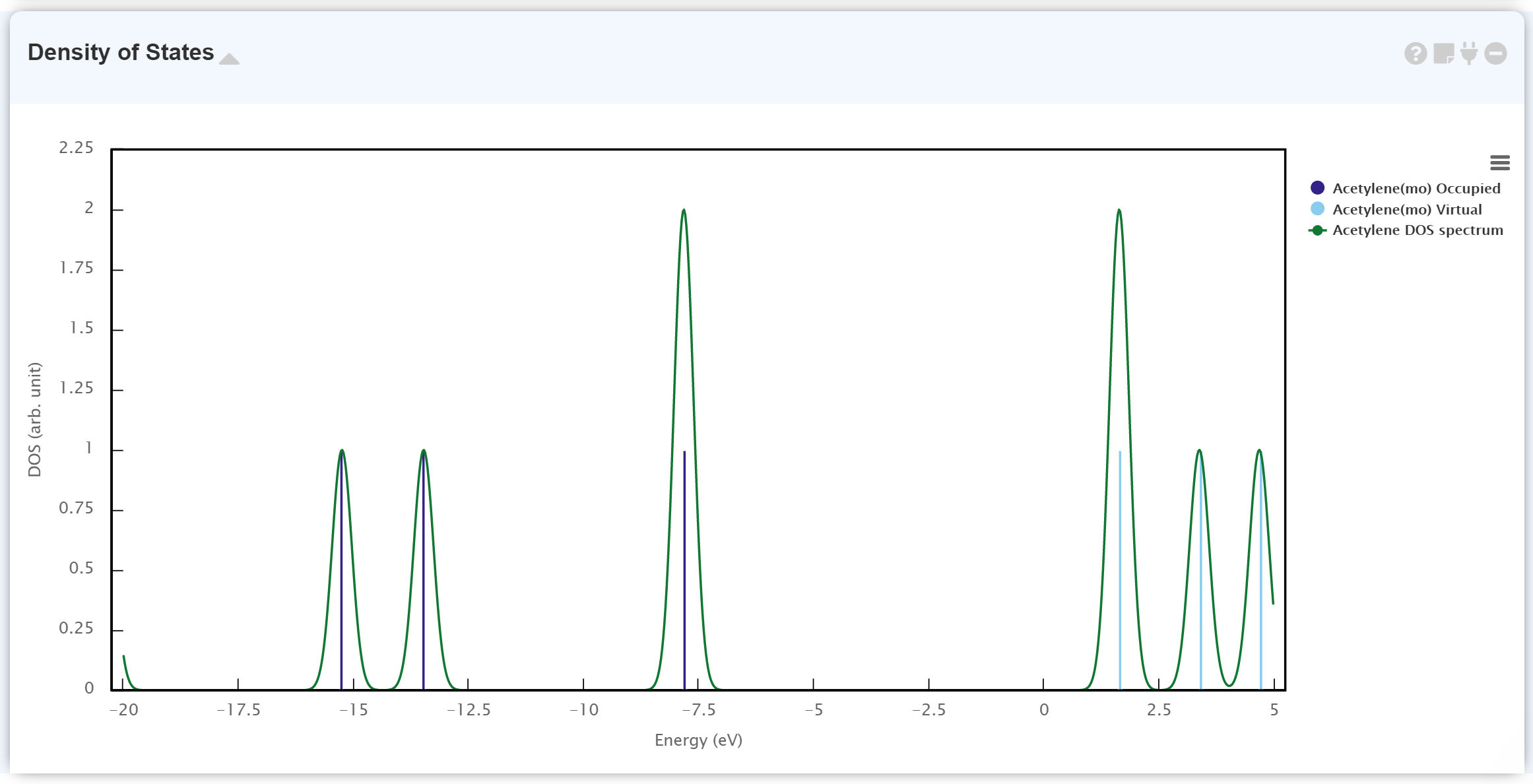
The Density of State module plots the calculated electronic status. The discontinuous graph is for MO eigenvalues; the dark-blue and light-blue lines correspond to occupied MO and virtual (unoccupied) MO, respectively. The continuous graph ([Job Name] DOS spectrum) is the Gaussian broadening data from the MO eigenvalue.
It is beneficial to combine the 'Density of States' module and the 'Surface' module for more detailed information of each MO.
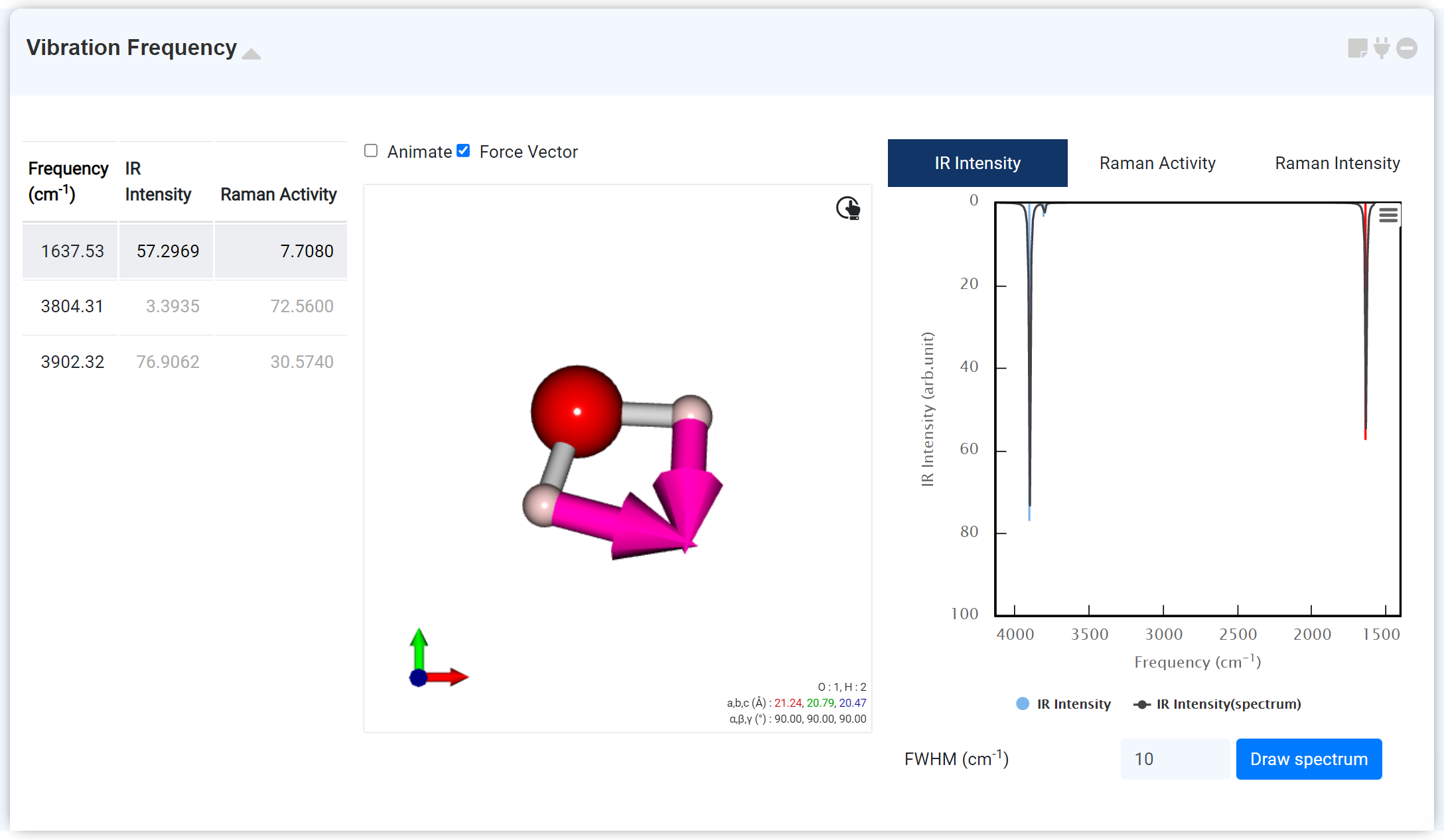
The 'Vibration Frequency' module displays the 'IR frequency' and ' Raman activity' data obtained from the GAMESS module. Within the GAMESS module, the 'IR frequency' can be obtained through the 'IR frequency option: True' of '&STATPT' when 'RUN Type: OPTIMIZE.' The 'Raman activity' can be calculated by setting 'RUN Type: RAMAN' on the new GAMESS module, which is connected to the previous module performing the hessian calculation.
You can check the following data from the 'Vibration Frequency' module:
- List of the vibrational modes
- Frequency information of the vibrational mode
- Vibrational mode animation
- Force vector (Arrow)
- IR Intensity
- Raman Activity
- Raman Intensity
You can change the FWHM of the spectrum (Full Width at Half Maximum, expressed in units of cm-1) at the bottom. For the Raman Intensity, you can draw a new spectrum by changing the Excitation Wavelength and temperature.
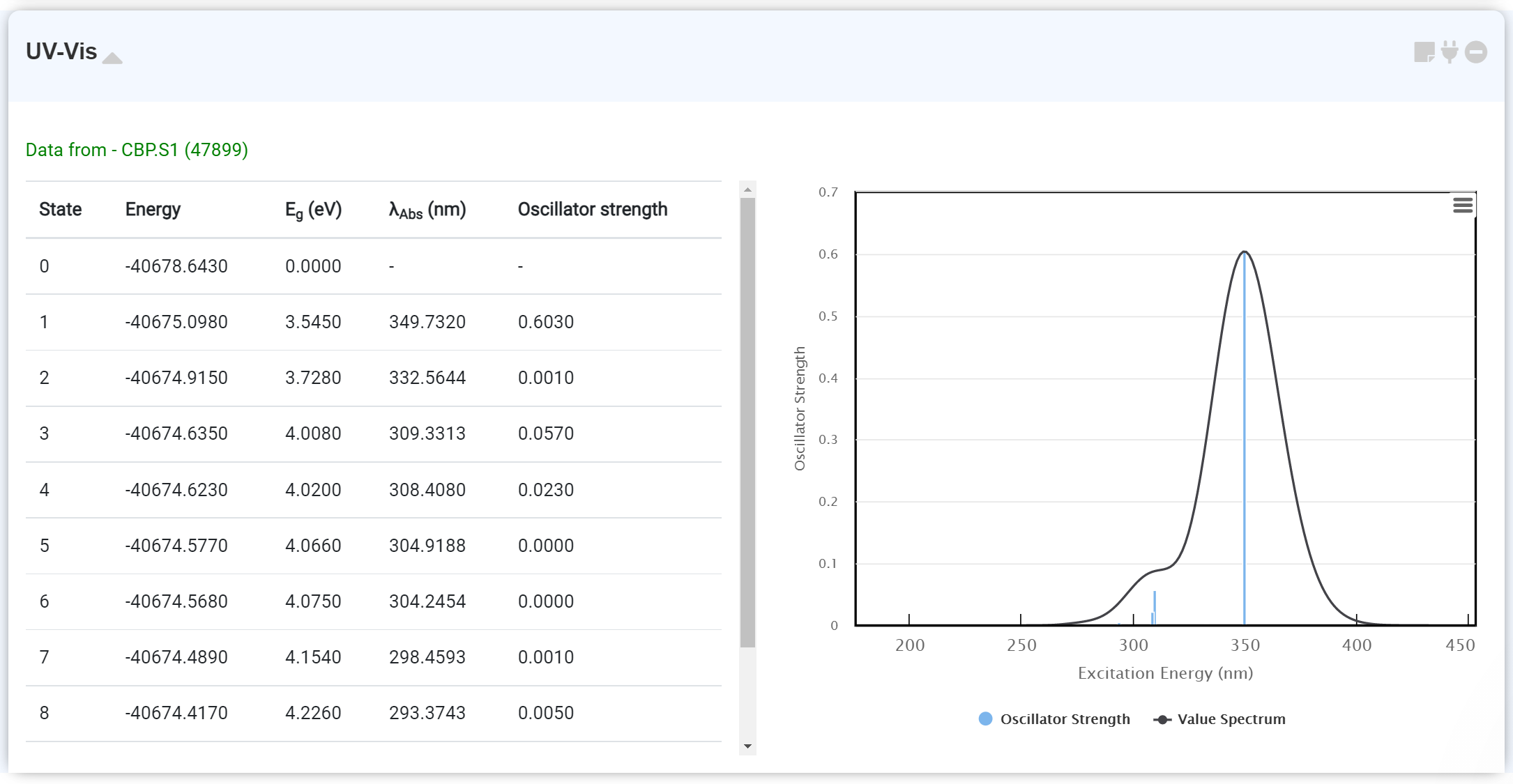
This module enables to check the UV/Vis spectrum calculation data. You can obtain the UV/Vis spectrum data on the GAMESS module by turning on the 'TDDFT: EXCITE' option. It is recommended to perform the excitation state calculation after finishing the optimization calculation. Connect the newly added GAMESS module with the first module, which performs this initial optimization. At this point, you should also set the 'RUN Type' as 'ENERGY'.
By hovering the mouse pointer on the spectrum, you can check the λAbs and Oscillator Strength.
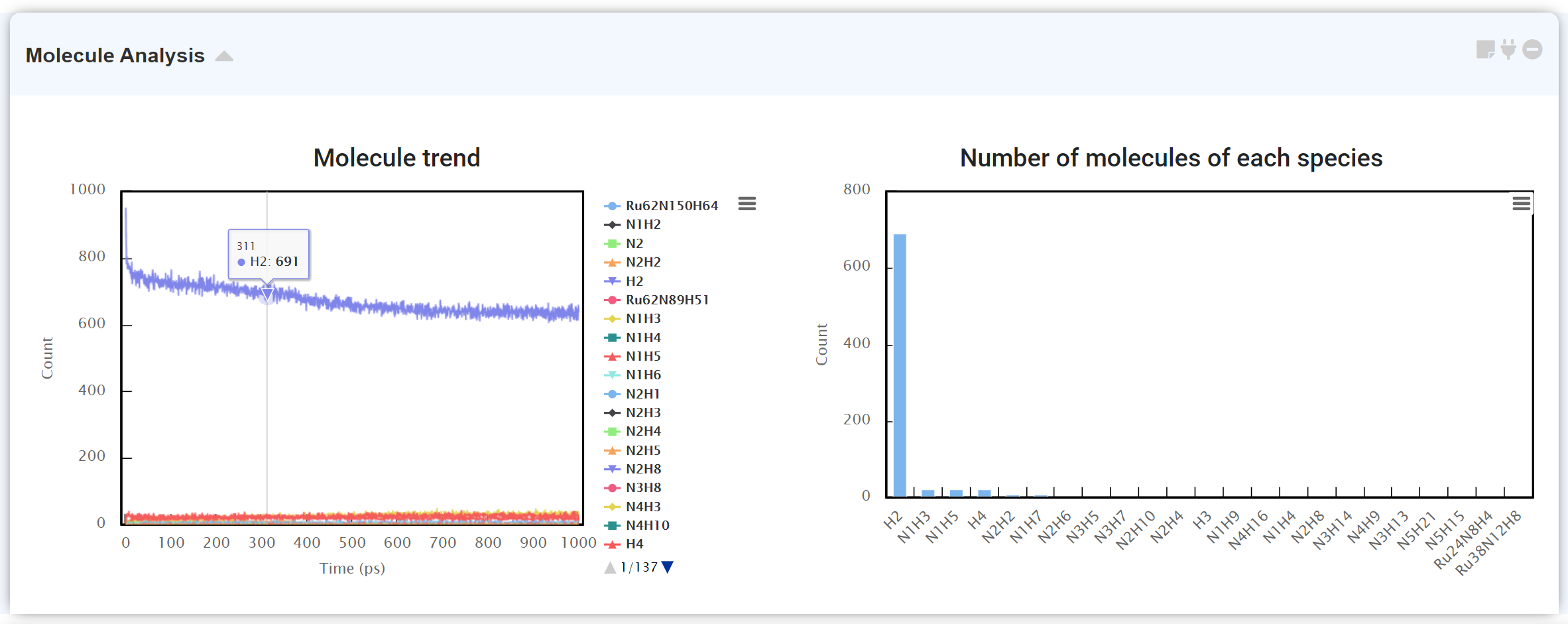
“Molecule Analysis” module counts number of atoms after molecular dynamics simulation. It displays the number of molecules existing in the system with respect to time by analyzing (left), and counting the number of atoms for the chemical species to find what molecule exists majorly at the time (right).
It may take some time if there are many atoms in the system.
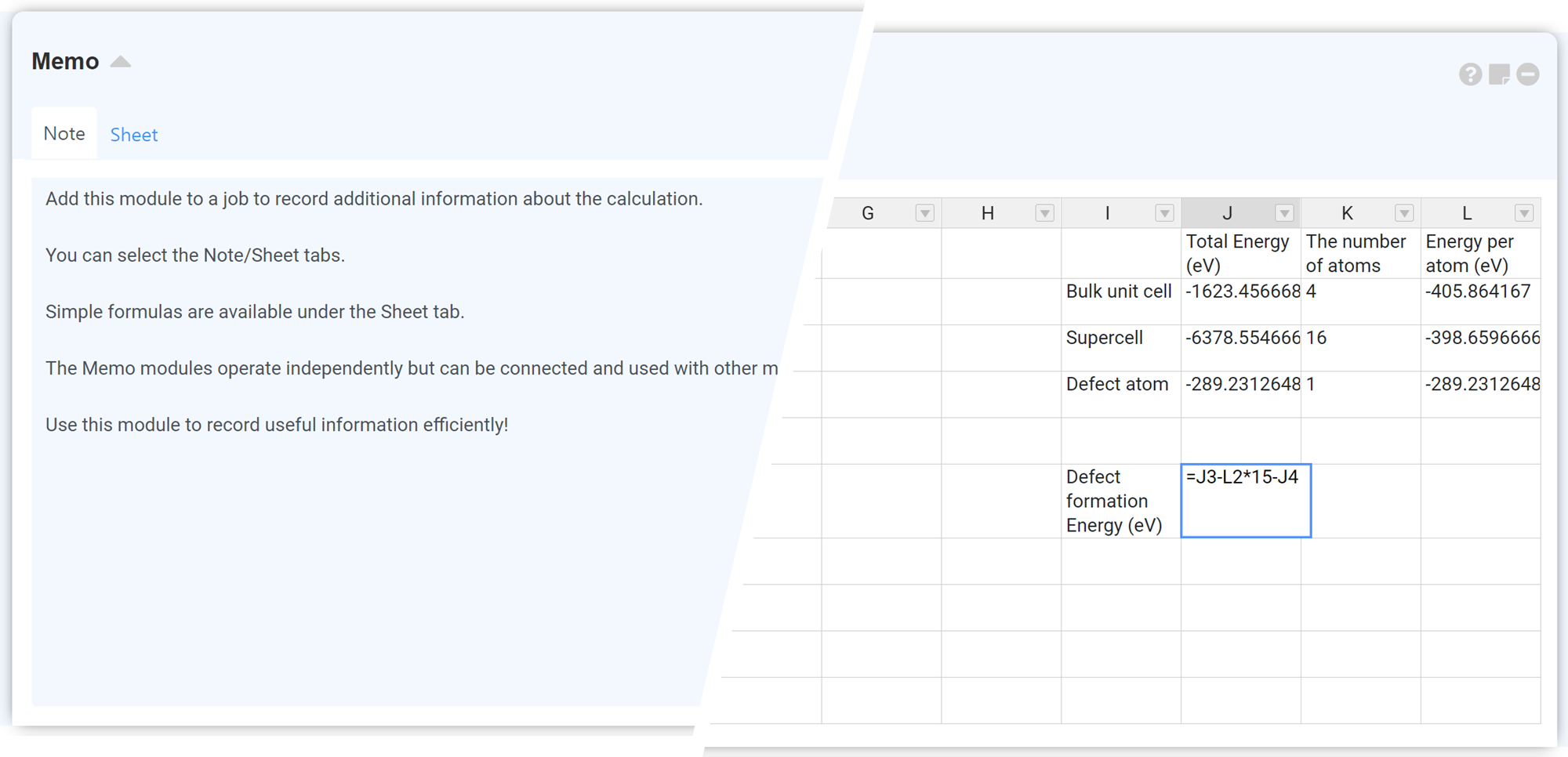
The 'Sheet' tab used the the Formulas plugin of Handsontable. For further information, please refer to the Handsontable Formula Support.
Features:
- Any numbers, negative and positive as float or integer;
- Arithmetic operations such as:
+,-,/,*,%,^; - Logical operations such as:
AND(),OR(),NOT(),XOR(); - Comparison operations such as:
=,>,>=,<,<=,<>; - All JavaScript Math constants such as:
PI(),E(),LN10(),LN2(),LOG10E(),LOG2E(),SQRT1_2(),SQRT2(); - Error handling:
#DIV/0!,#ERROR!,#VALUE!,#REF!,#NAME?,#N/A,#NUM!; - String operations such as:
&(concatenation eq.=-(2&5)will return-25); - All excel formulas defined in formula.js;
- Relative and absolute cell references such as:
A1,$A1,A$1,$A$1; - Build-in variables such as:
TRUE,FALSE,NULL; - Custom variables;
- Nested functions;
- Dynamic updates.
Known limitations:
- Not working with filtering and column sorting;
- Not working with trimming rows.