MatSQ provides a tutorial video for users who are not familiar with the service.
How would you simulate materials used in your research with DFT? DFT can compute electronic structures for only a few to dozens of models because of the limitations of computing performance. Periodic boundary conditions were introduced as a way of overcoming these limitations and simulating a bulk condition similar to the macroscopic system. In periodic boundary conditions, a material is defined as follows:
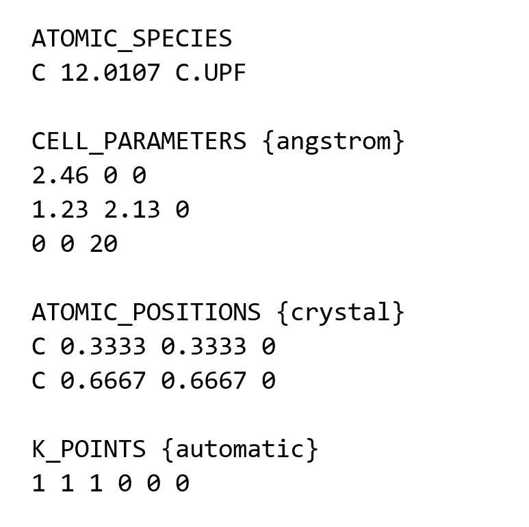
In periodic boundary conditions, a structure is repeated infinitely, so a silicon unit cell with eight atoms, a silicon supercell with 32 atoms, and a silicon bulk are theoretically identical. Moreover, because atoms are repeated by the space-group rules within the unit cell, silicon unit cells can be modeled only with the following information:
The computer recognizes a calculation model with a view that the structure shown on Structure Builder is repeated infinitely. If the cell size increases because of increased vacuum, the vacuum is recognized as repetitive, and the calculation is performed in the vacuum space too, so the amount of computation also increases. Roughly speaking, computational cost is proportional to V N (2 < N < 3), as the number of basis functions (plane waves) proportional to the volume of periodic unit cell. If you add a vacuum to model an atom, molecule, or slab structure, it is appropriate to have 10 to 15 Å clearance with the next repetitive model. You can check the repetitive structure by ticking "Ghost" in the right-click menu in the Visualizer Canvas of Structure Builder.
You can obtain the information or structure file required for unit cell modeling at the following link:
The following section gives a brief introduction to Quantum Espresso (QE), one of the DFT codes available on Materials Squire to run materials simulations. To understand in detail how Quantum Espresso works and what it can do, we recommend reading the documentation provided at www.quantum-espresso.org.
Quantum Espresso is an integrated suite of open-source computer codes for electronic-structure calculations and materials modeling at the nanoscale. It is based on the density-functional theory (DFT), plane waves, and pseudopotentials.
- The Quantum Espresso package is an expandable distribution of related packages. Two core packages for DFT electronic structure calculations, PWscf (Plane Wave self-consistent field), and CP (Car-Parrinello Molecular Dynamics) are supplemented by various packages for specialized applications as well as plug-ins. For more information on all packages, refer to the Quantum Espresso official user guide .
- Quantum Espresso provides open-source software packages. This means that everyone can study, expand, and modify the source code, allowing for continuous improvement.
- The theory behind Quantum Espresso’s algorithm for electronic structure calculations and materials modeling is determined by the Kohn-Sham density functional theory (KS-DFT). In other words, the code implements the common iterative self-consistent method to solve the Kohn-Sham equations.
- To perform materials simulations by a computer, we must expand functions like the wave function or the electron density in a basis set. Quantum Espresso uses plane waves as a basis set under the Bloch’s theorem. For the Gamma point, it is a Fourier series expansion of functions. A finite number of expansion coefficients, which is required for computation, can be achieved by an energy cutoff (ecutwfc, ecutrho).
- Pseudopotentials are used to smoothen the Coulomb potential by atomic nucleis, resulting in fewer plane waves, without affecting the result too much. Quantum Espresso allows the use of various pseudopotentials (norm-conserving, ultrasoft, PAW). Choosing the pseudopotential for a given system is a science in itself. Refer to the Quantum Espresso documentation for further information.
Based on DFT, Quantum Espresso has numerous applications, ranging from ground-state energy calculations and structural optimization to molecular dynamics as well as the modeling of response and spectroscopic properties. DFT simulations can be done on any crystal structure or supercell, which features some form of periodicity. Furthermore, Quantum Espresso works for insulators, semiconductors, and metals, offering different options for k-point sampling as well as smearing of energy states. To speed up computations, Quantum Espresso can deal with various pseudopotentials and approximate exchange-correlation functionals. For more information, visit the Quantum Espresso website .
The Quantum Espresso input script contains all information about the system of interest and defines the calculation process. The information consists of the namelist and input_cards. The following figure shows the general syntax of the input script.
There are three mandatory namelists in the PWscf package:
- It lists input variables that control the calculation process or determine the number of I/O. Examples include the calculation type, information amount (verbosity), and directory.
- It includes input variables that determine the calculation system such as the number of atoms, Bravais lattice index, cutoff energies, and smearing methods.
- It controls the algorithms used to reach the self-consistent solution of Kohn-Sham equations. Examples include the convergence threshold for self-consistency and mixing beta.
- If the nuclei of the system are allowed to move in a calculation, this namelist contains necessary variables to control their motion. Variable atomic positions occur in molecular dynamics or structural relaxation computations.
- Similar to &IONS, this namelist must be included for calculations with variable cell dimensions.
For some input data, such as atomic coordinates, it is inconvenient to write it in the namelist syntax. To make life easier, Quantum Espresso, therefore, features input_cards that allow you to enter data in a more practical format. There are three mandatory input_cards to be entered:
- Lists the name, mass, and PP of the atomic species included in a calculation model
- Lists the name and coordinates of all atoms in a calculation model
- Refers to the k-point grid and shift information, which are used to determine the number of k-points to be sampled in each lattice direction
The following links might be helpful to learn more about Quantum Espresso:
| Parameter | Value | Description | |
|---|---|---|---|
| Calculation type | scf | It performs self-consistent field calculations without affecting the atoms’ position. Namelists &IONS and &CELL are ignored in calculations. An iterative solution process runs to calculate the total energy, forces, and stresses. | |
| relax | In a relax calculation, the atoms are allowed to move to find their minimum energy (structural optimization). Includes geometric optimization steps and iterative self-consistent field calculations. | ||
| vc-relax | It optimizes the structure for the atom position and the cell. The cell shape (angles, lattice constants) may change to find the optimized structure. It also includes geometric optimization steps and iterative self-consistent field calculations. | ||
| (vc-)md | It calculates molecular dynamics with DFT. (ab-initio MD, AIMD) | ||
| restart | nscf | It performs non-scf calculations. Using this scheme, you make a single step calculation with the superposition of atomic orbitals. In contrast with the scf calculation, unoccupied electron states are also considered. Therefore, an nscf calculation is an economical choice for calculations that require a large k-point sampling. | |
| bands | It calculates only the Kohn-Sham states for the given set of k-points. | ||
| Max scf steps | It determines the maximum number of scf algorithm runs until convergence is reached (scf is fixed to 1 unconditionally). | ||
| Information amount | low | Default | |
| high | It adds detailed information about k-points or the character table to a job.stdout file. | ||
| Force threshold | It is the convergence threshold for the force to an ionic minimization. Any force for all elements must be less than this value (3.8E-4 Ry/Bohr = 0.01 eV/Å ). | ||
| Time step | It sets the time step for an MD simulation (atomic unit, 1 a.u. = 4.8378*10^-17 s). | ||
| Parameter | Value | Description |
|---|---|---|
| occupations | smearing | It performs Gaussian smearing of occupation numbers on the assumption that an electron would occupy up to a point slightly above the balance band (suitable for metals). |
| fixed | It calculates without smearing on the assumption that the structure is an insulator. | |
| tetrahedra | The tetrahedron method (P.E. Bloechl, PRB 49, 16223 (1994)) is used, which is suitable for DOS calculations. It must use a Monkhorst’s pack (automatic) k-point. | |
| Ecut(wfc) | It is the kinetic energy cutoffs for wave functions. | |
| Ecut(rho) | It is the kinetic energy cutoffs for charge densities and potentials. The default value is "ecutrho = 4*ecutwfc". Norm-conserving potentials and ultrasoft pseudopotentials require a higher ecut (rho) (about 8 to 12 times ecutwfc). | |
| Gaussian broadeing | It is the value required for Gaussian spreading in the Brillouin zone (broadening similar to '0.002 Ry = 27E-3eV = approx.300 K'). | |
| Number of electron spin | 1 (all up) | It calculates without considering the spin. |
| 2 (up, down) | It calculates taking into account the spin polarization. The amount of calculation doubles the case of "nspin=1." | |
| 4 (Noncolinear) | It is used in noncollinear cases. | |
| Van der Walls correction | It is used to compensate data for models that are significantly affected by the Van der Waals force, such as a layered structure. | |
| grimme-d2 (DFT-D) | It corrects by the semi-empirical Grimme’s DFT-D2 method (S. Grimme, J. Comp. Chem. 27, 1787 (2006), V. Barone et al., J. Comp. Chem. 30, 934 (2009)). | |
| grimme-d3 (DFT-D3) | It corrects by the semi-empirical Grimme’s DFT-D3 method (S. Grimme et al., J. Chem. Phys 132, 154104 (2010)). | |
| tkatchenko-scheffler | It corrects the Tkatchenko-Scheffler dispersion with the C6 coefficient induced by the first principles (A. Tkatchenko and M. Scheffler, PRL 102, 073005 (2009)). | |
| XDM | It performs corrections with the exchange-hole dipole-moment model (A. D. Becke et al., J. Chem. Phys. 127, 154108 (2007), A. Otero de la Roza et al., J. Chem. Phys. 136, 174109 (2012)). | |
| Hubbard_U | the U parameter for the element of interest. | |
| Parameter | Value | Description |
|---|---|---|
| Max iteration step | Within an scf step, it sets the maximum step value for iteration, which continues until the convergence is completed. It is recommended to increase this value for structures with poor convergence. | |
| Mixing beta | The rate at which the final electron density is mixed with the initial electron density under the scf algorithm. It is recommended to decrease this value for structures with poor convergence. | |
| Convergence threshold | The value that sets the convergence threshold, which is the limit of the energy difference before and after an scf step. | |
| Mixing mode | plain | The Broyden charge density mixing method |
| TF | It adds a simple Thomas-Fermi screening (applicable to highly consistent systems). | |
| local-TF | It screens TF depending on the local density (applicable to highly consistent systems). | |
| Starting wavefunction | atomic | It starts wave function calculations from the superposition of atomic orbitals. Calculations are performed normally in most cases, but some fail occasionally. |
| atomic+random | In addition to the superposition of atomic orbitals, it considers random wave functions. | |
| random | It starts a calculation with random wave functions. It has a slower but safer start of scf. | |
| Parameter | Value | Description | |
|---|---|---|---|
| Ion dynamics | It specifies the algorithm in Structural Relaxation to consider atomic movement. | ||
| relax | bfgs | It uses the BFGS quasi-newton algorithm for structural relaxation; cell_dynamics must be "bfgs" too. (Default). | |
| damp | It uses damped (quick-min Verlet) dynamics for structural relaxation. | ||
| vc-relax | bfgs | It uses BFGS quasi-newton algorithm; cell_dynamics must be "bfgs" too. | |
| damp | It uses damped (Beeman) dynamics for structural relaxation | ||
| md | verlet | It uses the Verlet algorithm to integrate Newton’s equation (Default). | |
| langevin | The ion dynamics is the overdamped Langevin. | ||
| langevin-smc | The overdamped Langevin with Smart Monte Carlo (R.J. Rossky, JCP, 69, 4628 (1978)). | ||
| vc-md | beeman | It uses Beeman’s algorithm to integrate Newton’s equations (Default). | |
| upscale | It reduces conv_thr by conv_thr/upscale during structural optimization to increase accuracy when the relaxation approaches convergence (available in the bfgs option only). | ||
| Ion temperature | (vc-)md | not_controlled | It does not control ionic temperatures (Default). |
| rescaling | It controls ionic temperatures via velocity rescaling (first method). | ||
| md | rescale-v | It controls ionic temperatures via velocity rescaling (second method). | |
| rescale-T | It controls ionic temperatures via velocity rescaling (third method). | ||
| reduce-T | It reduces ionic temperatures for every nraise step by the ΔT value. | ||
| berendsen | It controls ionic temperatures with "soft" velocity rescaling. | ||
| andersen | It controls ionic temperatures with the Andersen thermostat method. | ||
| initial | It initializes ion temperatures to the starting temperature and leaves uncontrolled further on. | ||
| Starting temperature (K) | The starting temperature in MD simulations. | ||
| ΔT | Ion temperature = "rescale-T": At each step, the instantaneous temperature is multiplied by ΔT.
Ion temperature = "reduce-T": In every "nraise" step, the instantaneous temperature is reduced by ΔT. |
||
| nraise | It rescales the instantaneous temperature (https://www.quantum-espresso.org/Doc/INPUT_PW.html#idm938). | ||
| Parameter | Value | Description |
|---|---|---|
| Cell dynamics | It specifies the type of algorithms for variable cell relaxations to control the cell size. | |
| bfgs | The BFGS quasi-newton algorithm; ion_dynamics must be "bfgs" too. | |
| none | no dynamics | |
| sd | It is the steepest descent (not implemented). | |
| damp-pr | It is the damped (Beeman) dynamics of the Parrinello-Rahman extended lagrangian. | |
| damp-w | It is the damped (Beeman) dynamics of the new Wentzcovitch extended lagrangian. | |
| Cell factor | It is the maximum strain ratio of the cell size. | |
| Press threshold | It is the convergence threshold of the pressure applied to cells (Kbar). | |
| Parameter | Value | Description | |
|---|---|---|---|
| Sampling | automatic | It is an option to sample k-points in the Monkhorst-Pack method. It also distributes the k-point grid evenly to the supercell. | |
| GAMMA | It is similar to automatic 1x1x1 in that only one k-point is sampled, but there is a difference: the k-point is recognized as real rather than a complex number. It has the benefit of fast calculation. | ||
| crystal(_b) | It designates the k-point as the relative coordinates to the reciprocal lattice vector. If the last column of data is {crystal}, it represents the weight for each k-point. If the last column of data is {crystal_b}, it represents the k-point number to be sampled by the next crystal coordination. | ||
| # k-points | It is the number of k-points in the direction of the three lattice vectors, respectively. | ||
| shift | It shifts the k-point grid with respect to the origin. Depending on the symmetry of the supercell, shifting the k-points could lead to better results. | ||
| crystal(_b) | Path | You can use a high-symmetric point to set the path for k-point sampling. You have to enter the weight. | |
| weight | crystal: the weight for each k-point to have
crystal_b: the number of k-points to be sampled until the next k-point |
||
| Option | Description |
|---|---|
| ngauss | Type of gaussian broadening |
| degauss | Decide how much Gaussian Broadening will be done. You should note that the unit is Ry, not eV! |
| DeltaE | Energy grid step (eV) |
| Emin | Minimum of energy (eV) for DOS plot |
| Emax | Maximum of energy (eV) for DOS plot |
| Option | Description |
|---|---|
| spin_component | Detemine the kind of spin when plotting the Band structure. In this time, the 'Spin-down' option can be selected when you performed the spin-polarized calculation. |
| lsym | The bands will be classified according to the irreducible representation with considering the symmetry of k-points, if it set as '.TRUE.'. |
| Section | Option | Description |
|---|---|---|
| &INPUTPP | Data to plot | Detemine the data to obtain from the pp.x calculation. For further information, please refer to the link. https://www.quantum-espresso.org/Doc/INPUT_PP.html#idm24 |
| Planar/Macroscopic Average | The number of points | Set the density of datapoint of the result graph. |
| The size of the window | Determine the number of the slab. |
| Section | Option | Value | Description |
|---|---|---|---|
| &INPUTPP | calculation | eps | Compute the complex macroscopic dielectric function, at the RPA (Random phase approximation) level, neglecting local field effects. eps is computed both on the real or imaginary axis. |
| jdos | Compute the optical joint density of states. | ||
| &ENERGY_GRID | Broadening | Gaussian | Apply the gaussian broadening. |
| Lorentzian | Apply the Lorentzian broadening. | ||
| Inter-band Broadening (eV) | Determine the broadening parameter | ||
| Intra-band Broadening (eV) | Determine the broadening parameter | ||
| Frequency Range (eV) | Determine the Frequency range | ||
| Frequency Mesh | Set the number of datapoints | ||
| Optional Rigid Shift | Give shift when calculating the transition energy. | ||
This is the entire list of functions available in Quantum Espresso. Put 'Short name' in the DFT Functional input field.
| Short name | Complete name | Short description | References |
|---|---|---|---|
| pz | sla+pz | Perdew-Zunger LDA | J.P.Perdew and A.Zunger, PRB 23, 5048 (1981) |
| bp | b88+p86 | Becke-Perdew grad.corr. | |
| pw91 | sla+pw+ggx+ggc | PW91 (aka GGA) | J.P.Perdew and Y. Wang, PRB 46, 6671 (1992) |
| blyp | sla+b88+lyp+blyp | BLYP | C.Lee, W.Yang, R.G.Parr, PRB 37, 785 (1988) |
| pbe | sla+pw+pbx+pbc | PBE | J.P.Perdew, K.Burke, M.Ernzerhof, PRL 77, 3865 (1996) |
| revpbe | sla+pw+rpb+pbc | revPBE (Zhang-Yang) | Zhang and Yang, PRL 80, 890 (1998) |
| pw86pbe | sla+pw+pw86+pbc | PW86 exchange + PBE correlation | |
| b86bpbe | sla+pw+b86b+pbc | B86b exchange + PBE correlation | |
| pbesol | sla+pw+psx+psc | PBEsol | J.P. Perdew et al., PRL 100, 136406 (2008) |
| q2d | sla+pw+q2dx+q2dc | PBEQ2D | L. Chiodo et al., PRL 108, 126402 (2012) |
| hcth | nox+noc+hcth+hcth | HCTH/120 | Handy et al, JCP 109, 6264 (1998) |
| olyp | nox+lyp+optx+blyp | OLYP | Handy et al, JCP 116, 5411 (2002) |
| wc | sla+pw+wcx+pbc | Wu-Cohen | Z. Wu and R. E. Cohen, PRB 73, 235116 (2006) |
| sogga | sla+pw+sox+pbec | SOGGA | Y. Zhao and D. G. Truhlar, JCP 128, 184109 (2008) |
| optbk88 | sla+pw+obk8+p86 | optB88 | |
| optb86b | sla+pw+ob86+p86 | optB86 | |
| ev93 | sla+pw+evx+nogc | Engel-Vosko | Engel-Vosko, Phys. Rev. B 47, 13164 (1993) |
| tpss | sla+pw+tpss+tpss | TPSS Meta-GGA | J.Tao, J.P.Perdew, V.N.Staroverov, G.E. Scuseria, PRL 91, 146401 (2003) |
| m06l | nox+noc+m6lx+m6lc | M06L Meta-GGA | Y. Zhao and D. G. Truhlar, JCP 125, 194101 (2006) |
| tb09 | sla+pw+tb09+tb09 | TB09 Meta-GGA | F Tran and P Blaha, Phys.Rev.Lett. 102, 226401 (2009) |
| pbe0 | pb0x+pw+pb0x+pbc | PBE0 | J.P.Perdew, M. Ernzerhof, K.Burke, JCP 105, 9982 (1996) |
| b86bx | pb0x+pw+b86x+pbc | B86bPBE hybrid | |
| bhahlyp | pb0x+pw+b88x+blyp | Becke half-and-half LYP | |
| hse | sla+pw+hse+pbc | Heyd-Scuseria-Ernzerhof (HSE 06, see note below) | Heyd, Scuseria, Ernzerhof, J. Chem. Phys. 118, 8207 (2003); Heyd, Scuseria, Ernzerhof, J. Chem. Phys. 124, 219906 (2006). |
| b3lyp | b3lp+b3lp+b3lp+b3lp | B3LYP | P.J. Stephens,F.J. Devlin,C.F. Chabalowski,M.J. Frisch, J.Phys.Chem 98, 11623 (1994) |
| b3lypv1r | b3lp+b3lpv1r+b3lp+b3lp | B3LYP-VWN1-RPA | |
| x3lyp | x3lp+x3lp+x3lp+x3lp | X3LYP | X. Xu, W.A Goddard III, PNAS 101, 2673 (2004) |
| vwn-rpa | sla+vwn-rpa | VWN LDA using vwn1-rpa parametriz | |
| gaupbe | sla+pw+gaup+pbc | Gau-PBE (also "gaup") | |
| vdw-df | sla+pw+rpb +vdw1 | vdW-DF1 | M. Dion et al., PRL 92, 246401 (2004); T. Thonhauser et al., PRL 115, 136402 (2015) |
| vdw-df2 | sla+pw+rw86+vdw2 | vdW-DF2 | Lee et al., Phys. Rev. B 82, 081101 (2010) |
| vdw-df-c09 | sla+pw+c09x+vdw1 | vdW-DF-C09 | |
| vdw-df2-c09 | sla+pw+c09x+vdw2 | vdW-DF2-C09 | |
| vdw-df-obk8 | sla+pw+obk8+vdw1 | vdW-DF-obk8 (optB88-vdW) | Klimes et al, J. Phys. Cond. Matter, 22, 022201 (2010) |
| vdw-df-ob86 | sla+pw+ob86+vdw1 | vdW-DF-ob86 (optB86b-vdW) | Klimes et al, Phys. Rev. B, 83, 195131 (2011) |
| vdw-df2-b86r | sla+pw+b86r+vdw2 | vdW-DF2-B86R (rev-vdw-df2) | |
| vdw-df-cx | sla+pw+cx13+vdW1 | vdW-DF-cx | K. Berland and P. Hyldgaard, PRB 89, 035412 (2014) |
| vdw-df-cx0 | sla+pw+cx13+vdW1+HF/4 | vdW-DF-cx-0 | K. Berland, Y. Jiao, J.-H. Lee, T. Rangel, J. B. Neaton and P. Hyldgaard, J. Chem. Phys. 146, 234106 (2017) |
| vdw-df2-0 | sla+pw+rw86+vdw2+HF/4 | vdW-DF2-0 | |
| vdw-df2-br0 | sla+pw+b86r+vdW2+HF/4 | vdW-DF2-b86r-0 | |
| vdw-df-c090 | sla+pw+c09x+vdw1+HF/4 | vdW-DF-C09-0 | |
| vdw-df-x | sla+pw+????+vdwx | vdW-DF-x, reserved Thonhauser, not implemented | |
| vdw-df-y | sla+pw+????+vdwy | vdW-DF-y, reserved Thonhauser, not implemented | |
| vdw-df-z | sla+pw+????+vdwz | vdW-DF-z, reserved Thonhauser, not implemented | |
| rvv10 | sla+pw+rw86+pbc+vv10 | rVV10 | R. Sabatini et al. Phys. Rev. B 87, 041108(R) (2013) |
This is a brief introduction to SIESTA, a first-principles calculation code that can be used in Materials Square to perform material simulations. To understand more about how SIESTA works and what it can do, see https://siesta-project.org/siesta/.
SIESTA is a program that can perform electronic structure calculations and molecular dynamics simulations of molecules and solids. SIESTA versions 4.0 and later are released under the terms of the GPL open source license.
SIESTA is the same DFT-based calculation module as the "Quantum Espresso", but there are two major differences.
- Unlike Quantum Espresso, which uses only Plan-Wave (PW), SIESTA uses plane waves and atomic basis functions (Basis set) to express electronic states. The electronic wave function is represented as a linear combination of atomic orbitals (LCAO), and the combined basis function use a plane wave to represent the entire space.
- SIESTA calculation using the supercell technique (a method of calculating a large system by dividing it into small cells), allows for larger-scale system calculations than Quantum Espresso.
| Parameter | Value | Description | Note |
|---|---|---|---|
| Calculation Type default = SCF |
Select the overall calculation type. | ||
| SCF | Perform electronic structure calculations with fixed cell sizes and atom positions. | ||
| Relax | Perform calculations to optimize the structure by fixing the cell size and moving the positions of the atoms. | ||
| VC-relax | Perform calculations to optimize the structure by changing the cell size and moving the positions of the atoms. | ||
| Phonon | Perform the phonon calculations which are calculations of vibration modes between atoms. | ||
| MD | Perform the Ab-Initio molecular dynamics (AIMD). | ||
| MD Type default = NVE |
Select the desired MD calculation type. | Enabled when Calculation Type=MD is selected. | |
| NVE (Verlet) | Perform AIMD simulation with standard Verlet algorithm. | ||
| NVT (Nose) | Perform AIMD simulation with temperature controlled by the Nosé thermostat algorithm. | ||
| NPE (PR) | Perform AIMD simulation with pressure controlled by the Parrinello-Rahman method. | ||
| NPT (Nose-PR) | Perform the AIMD with temperature controlled by means of a Nosé thermostat and pressure controlled by the Parrinello-Rahman method. | ||
| Anneal-Temp. | MD with annealing to a desired temperature. Reach a target temperature by velocity rescaling. | ||
| Anneal-Pressure | MD with annealing to a desired pressure. Reach a target pressure by scaling of the unit cell size and shape. | ||
| Anneal-Temp. & Pressure | MD with annealing to a desired temperature and pressure. Reach a target temperature and pressure by velocity rescaling and by scaling of the unit cell size and shape. | ||
| Max. optimization steps default = 500 |
Set the maximum number of steps in a structural optimization cycle. If the "Force Tolerance" value is reached before the maximum number of steps is reached, the structural optimization calculation will stop. | Enabled when Calculation Type=VC-relax or relax is selected. | |
| Force Tolerance (eV/Ang) default = 0.001 |
Set the force tolerance for structure optimization. If the maximum atomic force is less than this value, the calculation will stop. | Enabled when Calculation Type=VC-relax or relax is selected. | |
| Stress Tolerance (GPa) default = 0.01 |
Set the stress tolerance value for the cell size optimization calculation (vc-relax). If the maximum atomic force is smaller than "Force Tolerance" and the maximum stress component is smaller than "Stress Tolerance", the calculation will stop. | Enabled when Calculation Type = VC-relax is selected. | |
| External E Field default = OFF |
Specify an external electric field for the calculation. This option is performed only in calculations for molecules, chains, or slabs. The direction of the electric field must be set to be perpendicular to the bulk direction. (It is not possible to set the electric field for bulk structures such as dielectrics or ferroelectrics.) | ||
| Dipole Correction default = OFF |
This option causes the electric field required to compensate the dipoles of the system to be calculated at each iteration of the self-consistent cycle. This option is not available on a charged system (Netcharge $(\neq)$ 0). The dipole of the system is calculated via $(D = -e\int(r-r_{0})\delta\rho(r))$ where $(r_{0})$ is the dipole origin, and $(\delta\rho(r))$ is valence pseudocharge density minus the atomic valence pseudocharge densities. |
||
| Supercell Size default = 1,1,1 |
This creates a supercell by extending it by $(\pm n)$ in each direction for phonon calculation supercell. For example, if you set the x, y, and z values to 2,2,1, the total cell size will be 5$(\times)$5$(\times)$1. | Enabled when calculation Type=Phonon is selected. | |
| Displacement (Bohr) default = 0.04 |
Set the displacement to use for the computation of the force constant matrix for phonon calculations. | Enabled when calculation Type=Phonon is selected. | |
| Parameter | Value | Description | Note |
|---|---|---|---|
| Functional type default = GGA |
Select the exchange-correlation functional type to use for simulation. | ||
| LDA | Perform a Local Density Approximation (LDA) calculation. Potential File must be set to LDA type. | ||
| GGA | Perform a Generalized Gradient Approximation (GGA) calculation. Potential File must be set to GGA type. | ||
| VDW | Perform a van der Waals (VDW) calculation. The Potential File must be set up by the user. | ||
| Authors default = PBE |
Particular parametrization of the exchange-correlation functional. | ||
| CA | (= PZ): (Spin) local density approximation (LDA/LSD). Quantum Monte Carlo calculation of the homogeneous electron gas by D. M. Ceperley and B. J. Alder, Phys. Rev. Lett. 45,566 (1980), as parametrized by J. P. Perdew and A. Zunger, Phys. Rev B 23, 5075 (1981) |
Enabled when Functional Type=LDA is selected. | |
| PW92 | LDA/LSD, as parametrized by J. P. Perdew and Y. Wang, Phys. Rev B 45, 13244 (1992) | Enabled when Functional Type=LDA is selected. | |
| PW91 | Generalized gradients approximation (GGA) of Perdew and Wang. Ref: P&W, J. Chem. Phys. 100, 1290 (1994) | Enabled when Functional Type=GGA is selected. | |
| PBE | GGA of J. P. Perdew, K. Burke and M. Ernzerhof, Phys. Rev. Lett. 77, 3865 (1996) | Enabled when Functional Type=GGA is selected. | |
| revPBE | Modified GGA-PBE functional of Y. Zhang and W. Yang, Phys. Rev. Lett. 80, 890 (1998) | Enabled when Functional Type=GGA is selected. | |
| RPBE | Modified GGA-PBE functional of B. Hammer, L. B. Hansen and J. K. Norskov Phys. Rev. B 59, 7413 (1999) | Enabled when Functional Type=GGA is selected. | |
| PBEsol | Modified GGA-PBE functional of J. P. Perdew et al, Phys. Rev. Lett. 100, 136406 (2008) | Enabled when Functional Type=GGA is selected. | |
| BLYP | (=LYP) GGA with Becke exchange (A. D. Becke, Phys. Rev. A 38, 3098 (1988)) and Lee-Yang-Parr correlation (C. Lee, W. Yang, R. G. Parr, Phys. Rev. B 37, 785 (1988)), as modified by B. Miehlich, A. Savin, H. Stoll, and H. Preuss, Chem. Phys. Lett. 157, 200 (1989). | Enabled when Functional Type=GGA is selected. | |
| DRSLL | (=DF1) van der Waals density functional (vdW-DF) of M. Dion, H. Rydberg, E. Schröder, D. C. Langreth, and B. I. Lundqvist, Phys. Rev. Lett. 92, 246401 (2004), with the efficient implementation of G. Román-Pérez and J. M. Soler, Phys. Rev. Lett. 103, 096102 (2009) | Enabled when Functional Type=VDW is selected. | |
| LMKLL | (=DF2) vdW-DF functional of Dion et al (same as DRSLL) reparametrized by K. Lee, E. Murray, L. Kong, B. I. Lundqvist and D. C. Langreth, Phys. Rev. B 82, 081101 (2010) | Enabled when Functional Type=VDW is selected. | |
| KBM | dW-DF functional of Dion et al (same as DRSLL) with exchange modified by J. Klimes, D. R. Bowler, and A. Michaelides, J. Phys.: Condens. Matter 22, 022201 (2010) (optB88-vdW version) | Enabled when Functional Type=VDW is selected. | |
| BH | vdW-DF functional of Dion et al (same as DRSLL) with exchange modified by K. Berland and P. Hyldgaard, Phys. Rev. B 89, 035412 (2014) | Enabled when Functional Type=VDW is selected. | |
| VV | vdW-DF functional of O. A. Vydrov and T. Van Voorhis, J. Chem. Phys. 133, 244103 (2010) | Enabled when Functional Type=VDW is selected. | |
| Basis Size default = DZP |
Select the basis set to use for simulation. | ||
| SZ | Use single zeta basis. | ||
| DZ | Use double zeta basis. | ||
| SZP | Use single zeta basis plus polarization orbitals. | ||
| DZP | Use double zeta basis plus polarization orbitals. | ||
| Energy Shift (Ry) default = 0.02 |
Set the standard for orbital-confining radii of the first-zeta PAO. | ||
| Spin-polarization default = non-polarized |
Select the spin component of the simulation. | ||
| non-polarized | Perform a calculation with spin-degeneracy (only one component). | ||
| polarized | Perform a calculation with colinear spin (two spin components). | ||
| non-collinear | Perform a calculation with non-colinear spin (4 spin components), up-down and angles. This calculation requires you entering the spin component in manual mode. | ||
| spin-orbit | Perform a calculation with spin-orbit coupling. This requires the pseudopotentials to be relativistic. | Relativistic pseudopotentials must be used. | |
| Net Charge (e) default = 0 |
Specify the net charge of the system. For example, the $(F^{-})$ ion would have NetCharge -1 , and the $(Na^{+})$ ion would have NetCharge 1. | ||
| Spin Fix default = False |
Choose whether to fix the spin value of the system. | Enabled when Spin-polarization=polarized is selected. | |
| Total Spin default = 0 |
Define the value of the imposed total spin polarization of the system (in units of the electron spin, 1/2). | Enabled when Spin Fix=True is selected. | |
| Spin Option default = False |
Define the initial spin density for a spin polarized calculation atom by atom. The desired initial spin-polarization (real, positive for spin up, negative for spin down). | ||
| Parameter | Description | Note |
|---|---|---|
| SCF Must Converge default = TRUE |
This option stops the calculation if convergence is not achieved even after proceeding with the specified maximum number of SCF iterations. | |
| Mesh Cutoff (Ry) default = 300 |
Define the plane wave cutoff for the grid. | |
| Max. SCF Iterations default = 1000 |
Define the maximum number of SCF iterations. | |
| SCF DM Tolerance default = 0.00001 |
Define the tolerance of the Density Matrix. The SCF calculation will be considered complete when the maximum difference between the output and input of each element of the DM during an SCF cycle is smaller than SCF.DM.Tolerance. | |
| Mixing Weight default = 0.1 |
Define the mixing ratio of the electron density obtained in the previous step and the initial electron density in SCF cycle. | |
| Mixing History default = 6 |
Specify the number of previous SCF steps used to estimate the inputs used in the next SCF calculation. | |
| Electronic Temperature (K) default = 300 |
Specify the temperature of the Fermi-Dirac or Methfessel-Paxton distribution. It is particularly useful when calculating metallic systems, and in some cases to speed up the convergence of SCF calculations. |
| Parameter | Description | Note |
|---|---|---|
| Grid | Set the k-point sampling using Monkhorst's Pack method. Divide the reciprocal lattice space (Brillouin zone) into equal intervals as much as the set grid and sample the k-points corresponding to the lattice points. | |
| Shift default = OFF | This is an option to move the k-point grid based on the origin. (off: 0.0 0.0 0.0; on: 0.5 0.5 0.5) |
| Parameter | Description | Note |
|---|---|---|
| Length Time Step (fs) default = 1 |
Set the length of the time step of the AIMD simulation. | |
| MD Step default = 100 |
Set the final time step of the MD simulation. The final time of the AIMD will be Length Time Step*MD step. | |
| Initial Temp. (K) default = 300 |
Specifies the initial temperature for the AIMD simulation. Atoms are assigned random rates from the Maxwell-Boltzmann distribution along with their corresponding temperatures. | |
| Target Temp. (K) default = 300 |
Specifies the target temperature in the AIMD simulation. It is used in NVT, NPT using Nose thermostat or annealing calculations among MD types. | Enabled when MD Type=NVT, NPT, Anneal-Temp., or Anneal-Temp.&Pressure is selected. |
| Target Pressure (GPa) default = 1 |
Specifies the target pressure in the AIMD simulation. Useful for cell optimizations and constant-pressure molecular dynamics. | Enabled when Calculation Type=vc-relax or MD Type=NPE, NPT, Anneal-Pressure, or Anneal-Temp.&Pressure is selected. |
| Generalized Mass (Ry fs2) default = 100 |
Specifies the generalized mass of the Nose or Parrinello-Rahman variable. This determines the time scale of the Nose or Parrinello-Rahman variable dynamics, and its coupling to the physical system. | If MD Type=NVT, MD.NoseMass is specified, If MD Type=NPE, MD.ParrinelloRahmanMass is assigned. |
| Relaxation Time (fs) default = 100 |
Specifies the relaxation time to reach target temperature and/or pressure in annealing MD. Note that this is a "Relaxation Time", and as such it gives a rough estimate of the time needed to achieve the given targets. | Enable when MD Type=Anneal-Temp., Anneal-Pressure, or Anneal-Temp.&Pressure is selected. |
| Estimate of Bulk Modulus (Ry/Bohr3) default = 100 |
Specifies an estimate (may be rough) of the bulk modulus of the system. This is needed to set the rate of change of cell shape to reach target pressure in annealing MD. | Enable when MD Type=Anneal-Pressure, or Anneal-Temp.&Pressure is selected. |
| Parameter | Value | Description | Note |
|---|---|---|---|
| Charge Density (3D) | Post-processing option to view Charge Density and Potential as a 3D structures. | ||
| Total Charge Density | Total charge density, up/down spin charge density, and spin difference density are extracted as 3D structure files. | ||
| Local Charge Density | Local charge density, up/down spin charge density, and spin difference density are extracted as 3D structure files. | Only enable when LDOS post-processing is connected to a completed calculation. | |
| Total Electrostatic Potential | Electrostatic potential is extracted as 3D structure files. | ||
| Total Potential | Total potential is extracted as 3D structure files. | ||
| Macroscopic/Planar average (2D) | Post-processing option to view Charge Density and Potential as a 2D structures. MWhen calculating macroscopic average (nanosmoothing), the data is output at the value set by the user. The set values are written to the macroave.in file. |
||
| Charge Density | The macroscopic average and planar average of charge density are extracted as 2D graph. | ||
| Electrostatic Potential | The macroscopic average and planar average of electrostatic potential are extracted as 2D graph. | ||
| # of convolutions default=1 |
Select the number of square filter functions in the macroaverage (nanosmoothing). (1 = surfaces, 2= Interfaces and superlattices) | ||
| Length of the first step function (bohr) default=2.96687 |
First length for the filter function in macroscopic average. | ||
| Length of the second step function (bohr) default=2.96687 |
Second length for the filter function in macroscopic average | This setting is only affected when # of convolutions=2. | |
| Total number of electrons default=501 |
Sets the total number of electrons in the system. This value is only used for renormalization when calculating the macroscopic average (nanosmoothed ). | This setting is only affected when checking Charge Density as a 2D structure. | |
| Parameter | Description | Note |
|---|---|---|
| Minimum Energy (eV) default = -20 |
Set the minimum of the energy range for PDOS. | |
| Maximum Energy (eV) default = 10 |
Set the maximum of the energy range for PDOS. | |
| Broadening (eV) default = 0.1 |
Set the peak width (an energy) for broadening the eigenvalues. | |
| K-point | Set the interval to sample k-points with the same Monkhorst's Pack method as the general calculation and choose whether to shift the grid or not. For accurate analysis, it is recommended to increase it by about 2~3 times than in the General calculations such as vc-relax, relax, or SCF. |
| Parameter | Description | Note |
|---|---|---|
| Minimum Energy (eV) default = -0.5 |
Set the minimum of the energy range for LDOS. | |
| Maximum Energy (eV) default = 0 |
Set the maximum of the energy range for LDOS. |
| Parameter | Description | Note |
|---|---|---|
| Crystal System default = Cube |
Select the crystal system from which to sample the high-symmetric point. It is recommended to set it to the same crystal system as the calculation model used. | |
| Number of k-points default = 10 |
Specifies the number of gaps between each k-point in the grid vector direction. | |
| High symmetry points | You can set the K-point path directly. High symmetry points are added by clicking on each K-point. Default is set to the path of the crystal selected in the Crystal system. | |
| Band Lines | Shows the set high-symmetric K-point path and number of intervals. You can also make your own edits here. |
| Parameter | Value | Description | Note |
|---|---|---|---|
| Minimum Energy (eV) default = 0 |
Specifies the minimum of the energy range in which the frequency spectrum will be calculated. | ||
| Maximum Energy (eV) default = 20 |
Specifies the maximum of the energy range in which the frequency spectrum will be calculated. | ||
| Broadening (eV) default = 0.5 |
Specifies the Gaussian broadening to be applied to the frequency values. | ||
| Mesh point default = 4, 4, 2 |
Determine the mesh size used for the integration across the Brillouin zone. | ||
| Polarization Type default = polycrystal |
Select the type of polarization to be used in the calculation. | ||
| polycrystal | default | ||
| polarized | The electric field is applied in the direction set in Optical Vector. | ||
| unpolarized | Light propagates in the direction set in Optical Vector. | ||
| Optical Vector default = 0, 0, 1 |
Sets the vector direction for either the electric field (polarized) or light propagation (unpolarized). | Enable when Polarization Type = polarized or unpolarized is selected | |
This is a brief introduction to GAMESS, the first-principle calculation code available in Material Square. For more information on how GAMESS works and possible applications, refer the official manual at https://www.msg.chem.iastate.edu/gamess/
GAMESS is a program for ab initio molecular quantum chemistry. Briefly, GAMESS can compute SCF wavefunctions ranging from RHF, ROHF, UHF, GVB, and MCSCF. Correlation corrections to these SCF wavefunctions include Configuration Interaction, second order perturbation Theory, and Coupled-Cluster approaches, as well as the Density Functional Theory approximation. Excited states can be computed by CI, EOM, or TD-DFT procedures. Nuclear gradients are available, for automatic geometry optimization, transition state searches, or reaction path following. Computation of the energy hessian permits prediction of vibrational frequencies, with IR or Raman intensities. Solvent effects may be modeled by the discrete Effective Fragment potentials, or continuum models such as the Polarizable Continuum Model. Numerous relativistic computations are available, including infinite order two component scalar relativity corrections, with various spin-orbit coupling options.
A variety of molecular properties, ranging from simple dipole moments to frequency dependent hyperpolarizabilities may be computed. Many basis sets are stored internally, together with effective core potentials or model core potentials, so that essentially the entire periodic table can be considered.
Most computations can be performed using direct techniques, or in parallel on appropriate hardware.
This group specifies the type of wavefunction, the type of calculation, use of core potentials, spherical harmonics, coordinate choices, and similar fundamental job options.
| Parameter | Value | Description | |
|---|---|---|---|
| SCF Type | RHF (Default) | Restricted Hartree Fock calculation | |
| UHF | Unrestricted Hartree Fock calculation | ||
| ROHF | Restricted open shell Hartree-Fock. | ||
| MCSCF | Multiconfigurational SCF wavefunction | ||
| MPLEVL | Chooses Møller-Plesset perturbation theory level, after the SCF. See $MP2, or $MRMP for MCSCF. | ||
| 0 (Default) | Skip the MP computation | ||
| 2 | Perform second order energy correction. | ||
| RUN Type | ENERGY (Default) | Molecular energy without structure optimization | |
| HESSIAN | Molecular energy plus gradient plus second derivatives, including harmonic vibrational analysis. See the $FORCE and $CPHF input groups. | ||
| OPTIMIZE | Optimize the molecular geometry using analytic energy gradients. See $STATPT. | ||
| SADPOINT | Locate saddle point (transition state). See $STATPT. | ||
| RAMAN | computes Raman intensities, see $RAMAN. | ||
| DFT Type | NONE (Default) | ab initio computation (Hartree-Fock Method) | |
| BLYP | perform density functional theory run, using the functional specified. Please refer to the following link to look at the 'DFTTYP' tag description. https://www.msg.chem.iastate.edu/gamess/GAMESS_Manual/docs-input.txt | ||
| B3LYP | |||
| PBE | |||
| PBE0 | |||
| PW91 | |||
| REVPBE | |||
| TDDFT | NONE (Default) | no excited states | |
| EXCITE | generate time-dependent DFT excitation energies, using the DFTTYP= functional, for RHF or UHF references. Analytic nuclear gradients are available for RHF. See $TDDFT. | ||
| Charge | Total charge of the molecular system | ||
| 0 (Default) | Neutral | ||
| +1, -1, -2, ... | monovalent cation, monovalent anion, divalent anion, ... | ||
| Multiplicity | Multiplicity of the electronic state | ||
| 1 (Default) | Singlet | ||
| 2, 3, … | doublet, triplet, and so on. | ||
| ISPHER | Spherical Harmonics option | ||
| -1 (Default) | Use Cartesian basis functions to construct symmetry-adapted linear combination (SALC) of basis functions. The SALC space is the linear variation space used. | ||
| 0 | Use spherical harmonic functions to create SALC functions, which are then expressed in terms of Cartesian functions. The contaminants are not dropped, hence this option has EXACTLY the same variational space as ISPHER=-1. The only benefit to obtain from this is a population analysis in terms of pure s,p,d,f,g functions. | ||
| 1 | Same as ISPHER=0, but the function space is truncated to eliminate all contaminant Cartesian functions [3S(D), 3P(F), 4S(G), and 3D(G)] before constructing the SALC functions. The computation corresponds to the use of a spherical harmonic basis. | ||
| PP | NONE (Default) | All electron calculation | |
| SBKJC | Stevens/Basch/Krauss/Jasien/Cundari valence basis set, for Li-Rn. This choice implies an unscaled -31G basis for H-He. | ||
| HW | Hay/Wadt valence basis. This is a -21 split, available Na-Xe, except for the transition metals. This implies a 3-21G basis for H-Ne. | ||
| MCP | Select PP=MCP in $CONTRL to automatically use the model core potential matching your basis choice below. References for these bases, and other information about MCPs can be found in the REFS.DOC chapter. Another family covering almost all elements is available in $DATA only. | ||
| READ | Read ECP potentials in the $ECP input. | ||
This group allows certain standard basis sets to be easily requested. Basis sets are specified by several keywords: GBASIS, NDFUNC, BASNAM, etc.
| Parameter | Class | Value | Keywords | Description | Available Elements |
|---|---|---|---|---|---|
| BASIS | Semiempirical | AM1 | GBASIS=AM1 | selects AM1 model Hamiltonian | C, H, O, N |
| PM3 | GBASIS=PM3 | selects PM3 model Hamiltonian | H, C-F, Al-Cl, Br, I | ||
| Gaussian functions | STO-3G | GBASIS=STO NGAUSS=3 | Pople's STO-NG minimal basis set. | H-Xe | |
| 3-21G (Default) | GBASIS=N21 NGAUSS=3 | Pople's N-21G split valence basis set + 3 gaussian functions. | H-Xe | ||
| 6-31G* | GBASIS=N31 NGAUSS=6 NDFUNC=1 | Pople's N-31G split valence basis set + 6 gaussian functions and heavy atom polarization functions. | H-Kr | ||
| 6-311G** | GBASIS=N311 NGAUSS=6 NDFUNC=1 NPFUNC=1 | Pople's "triple split" N-311G basis set + 6 gaussian functions, heavy atom polarization functions, and p type polarization functions for light atom (H-He). | H-Ne | ||
| 6-311G**+ | GBASIS=N311 NGAUSS=6 NDFUNC=1 NPFUNC=1 DIFFSP=.TRUE. | Pople's "triple split" N-311G basis set + 6 gaussian functions, p type polarization functions for light atom (H-He), and polarizaiton function, diffuse function for heavy atoms. | H-Ne | ||
| Auxiliary basis set | cc-pVDZ | GBASIS=CCD | cc-pVDZ basis | H-Ar | |
| cc-pVTZ | GBASIS=CCT | cc-pVTZ basis | H-Ar | ||
| aug-cc-pVDZ | GBASIS=ACCD | aug-cc-pVDZ basis | H-Ar | ||
| Effective Core Potential (ECP) | SBKJC | GBASIS=SBKJC | Stevens/Basch/Krauss/Jasien/Cundari valence basis set, for Li-Rn. This choice implies an unscaled -31G basis for H-He. | H-Rn | |
| Custom | def2-svp | GBASIS=d2svp EXTFIL=.TRUE. | Custom basis set for heavy metal elements | H-Rn, La-Lu | |
| def2-tzvp | GBASIS=d2tzvp EXTFIL=.TRUE. | Custom basis set for heavy metal elements | H-Rn, La-Lu | ||
| LANL2DZ | GBASIS=lanl2dz EXTFIL=.TRUE. | Custom basis set for heavy metal elements | H-Bi, La, U-Pu | ||
| CUSTOM | GBASIS={User Define} EXTFIL=.TRUE. | Please refer to the following link to look at the 'GBASIS' tag description. https://www.msg.chem.iastate.edu/gamess/GAMESS_Manual/docs-input.txt You can download your custom basis set from Basis Set Exchange. https://www.basissetexchange.org/ | User Define |
This group controls the selection of initial molecular orbitals.
| Parameter | Value | Description |
|---|---|---|
| Initial Orbital | Write type of initial orbital guess. | |
| Huckel (Default) | Carry out an extended Huckel calculation using a Huzinaga MINI basis set, and project this onto the current basis. This is implemented for atoms up to Rn, and will work for any all electron or core potential basis set. (default for most runs) | |
| HCORE | Diagonalize the one electron Hamiltonian to obtain the initial guess orbitals. This method is applicable to any basis set, but does not work as well as the HUCKEL guess. | |
| MOREAD | Read in formatted vectors punched by an earlier run. This requires a $VEC deck, and you MUST pay attention to NORB below. | |
| RDMINI | Read in a $VEC deck from a converged SCF calculation using GBASIS=MINI, to project the MINI orbitals onto the current basis. The option improves upon the Huckel guess because it involves SCF orbitals, which are typically easily obtained in the small MINI basis. This option doesn't work if the current basis uses core potentials. potentials. The $VEC from the MINI run must contain all virtual orbitals. | |
| MOSAVED | (default for restarts) The initial orbitals are read from the DICTNRY file of the earlier run. | |
| SKIP | Bypass initial orbital selection. The initial orbitals and density matrix are assumed to be in the DICTNRY file. Mostly used for RUNTYP=HESSIAN when the hessian is being read in from the input. | |
This group controls solvent effect computations using the Polarizable Continuum Model.
The default calculation, chosen by selecting only the SOLVNT keyword, is to compute the electrostatic free energy. Appropriate numerical constants are provided for a wide range of solvents.
Additional keywords (ICOMP, ICAV, IDISP, or IREP/IDP) allow for more sophisticated computations, namely cavitation, repulsion, and dispersion free energies. The methodology for these is general, but numerical constants are provided only for water.
| Parameter | Value | Description | |
|---|---|---|---|
| Solvent effect | NONE (Default) | ||
| WATER | Water (H2O) | ||
| CH3OH | Methanol (CH3OH) | ||
| C2H5OH | Ethanol (C2H5OH) | ||
| CLFORM | Chloroform (CHCl3) | ||
| CTCL | Carbon Tetrachloride (CCl4) | ||
| METHYCL | Methylene Chloride (CH2Cl2) | ||
| 12DCLET | 1,2-Dichloroethane (CH2ClCH2Cl) | ||
| BENZENE | Benzene (C6H6) | ||
| TOLUENE | Toluene (C6H5CH3) | ||
| CYClOHEXANE | Cyclohexane (C6H12) | ||
| CUSTOM | ACETONE | Acetone (CH3COCH3) | |
| ANILINE | Aniline (C6H5NH2) | ||
| CLBENZ | Chlorobenzene (C6H5Cl) | ||
| DMSO | Dimethylsulfoxide (DMSO) | ||
| NEPTANE | N-Heptane (C7H16) | ||
| NITMET | Nitromethane (CH3NO2) | ||
| THF | Tetrahydrofuran (THF) | ||
This group controls the computation of the hessian matrix (the energy second derivative tensor, also known as the force constant matrix), and an optional harmonic vibrational analysis. This can be a very time consuming calculation. However, given the force constant matrix, the vibrational analysis for an isotopically substituted molecule is very cheap. Related input is HESS= in $STATPT, and the $MASS, $HESS, $GRAD, $DIPDR, $VIB inputs. Calculation of the hessian automatically yields the dipole derivative tensor, giving IR frequencies. Raman intensities are obtained by following with RUNTYP=RAMAN.
| Parameter | Value | Description |
|---|---|---|
| METHOD | chooses the computational method | |
| ANALYTIC (Default) | ANALYTIC is a fully analytic calculation. This is implemented for SCFTYP=RHF, UHF, ROHF, GVB (for NPAIR=0 or 1, only), and MCSCF (for CISTEP=ALDET or ORMAS, only). R-DFT and U-DFT are also analytic. | |
| SEMINUM | SEMINUM does numerical differentiation of analytically computed first derivatives. This is the default for UHF, MCSCF using other CISTEPs, all solvent models, relativistic corrections, and most MP2 or CI runs. | |
| FULLNUM | FULLNUM numerically differentiates the energy twice, which can be used by all other cases. It requires many energies (a check run will tell how many) and so it is mainly useful for systems with only very few symmetry unique atoms. | |
| Temperature (K) | 298.15 (Default) | An array of up to ten temperatures at which the thermochemistry should be printed out. The default is a single temperature, 298.15 K. To use absolute zero, input 0.001 degrees. |
This group controls the search for stationary points (ground state).
| Parameter | Value | Description |
|---|---|---|
| Convergence tolerance (Hartree/Bohr) | 0.0001 (Default) | Gradient convergence tolerance (unit: Hartree/Bohr) Convergence of a geometry search requires the largest component of the gradient to be less than OPTTOL, and the root mean square gradient less than 1/3 of OPTTOL. |
| Max iteration step | 500 (Default) | The maximum number of steps to take. Restart data is punched if NSTEP is exceeded. The default is 50 steps for a minimum search, but only 20 for a transition state search, which benefit from relatively frequent Hessian re-evaluations. |
| Hessian matrix | GUESS (Default) | GUESS chooses an initial guess for the hessian. (default for RUNTYP=OPTIMIZE) |
| CALC | Compute the hessian, see $FORCE input. | |
| IR frequency | Flag to control automatic hessian evaluation at the end of a successful geometry search. (default=.FALSE.) | |
This group generates molecular excitation energies by time-dependent density functional theory computations (or time-dependent Hartree-Fock, also known as the Random Phase Approximation).
| Parameter | Value | Description |
|---|---|---|
| Nstate | 10 (Default) | Number of states to be found (excluding the reference state). The default is 1 more state. |
| MULT | 1 (Default) | Multiplicity (1 or 3) of the singly excited states. This keyword applies only when the reference is a closed shell. This parameter is ignored when TDDFT=SPNFLP. |
This is a brief introduction to LAMMPS, the molecular dynamics code available in Material Square. For more information on how LAMMPS works and possible applications, refer the official manual at lammps.sandia.gov.
LAMMPS (Large-scale Atomic/Molecular Massively Parallel Simulator) is a classical molecular dynamics simulation code, developed at the Sandia National Laboratory, it designed to be calculated effectively with parallel computing. Base on Newton's equation of motion, LAMMPS can calculate a system consists of several hundred to several billion atoms using forcefield for fast speed. It can calculate not only the stability at the given temperature which is a basic property in the materials study, but also mechanical, thermal and chemical properties of material. Recently, the effectivity of parallel computing using the Graphics Processing Unit (GPU) was increased, and machine learning can be used for the expanding interatomic potential.
| Parameter | Value | Description |
|---|---|---|
| Reactive Forcefield | ID | The identification value of each reactive forcefield |
| Type | The type of reactive forcefield | |
| Elements | Elements for the reactive forcefield to consider | |
| Author | The author of the reactive forcefield | |
| DOI | The paper on the corresponding reactive forcefield | |
| Ensemble | NVT | An NVT ensemble is also known as the canonical ensemble. It assumes a calculation model as an isolated system, which has a fixed temperature, volume, and the number of atoms. |
| NVE | An NVE ensemble is also known as the microcanonical ensemble. This assumes a calculation model as an isolated system, which cannot exchange energy or particles with its environment because the energy of the system is fixed. | |
| After Relax | Before starting an MD simulation, a structural relaxation is performed at room temperature (200 K – 300 K) first for structural stabilization. It can reduce the probability that the calculation would fail because of structural instability. | |
| Dump | It saves the trajectory in a file for every step selected. For calculations with long simulation times, you can reduce the overall file size. | |
| Temperature | Begin (K) | The temperature at the start of a simulation |
| Final (K) | The target temperature during simulation | |
| Damping (Step) | Resets the temperature for each damping step | |
| Time (ps) | Specifies the total simulation time (1 ns = 1000 ps) | |
| Initial Velocity (Å/fs) | The initial speed of the atom group selected | |
| Force (Kcal/mole-Å) | The force per fs applied to the selected atom group | |
| Move (Linear, Å/fs) | The distance traveled per fs for the selected atom group | |
Please add citation by the URL to cite the Materials Square.
Please refer to Acknowledgement page to cite the simulation packages implemented in Materials Square.
The list shows the publications which applied the calculation results obtained by the calculation package implemented in Materials Square.
Please refer to Acknowledgement page to cite the simulation packages implemented in Materials Square.
The list shows the publications which applied the calculation results obtained by the calculation package implemented in Materials Square.
- Yoon, H., Song, H. J., Hyoung, J. S., Jung, S. W., Haryanto, A., Lee, C. W., & Kim, D. W. (2024). Facet-engineered ruthenium oxide on titanium oxide oxygen evolution electrocatalysts for proton-exchange membrane water electrolysis.Applied Catalysis B: Environment and Energy, 124382.
- Jang, K., Song, H. J., Park, J. B., Jung, S. W., & Kim, D. W. (2024). Magnesium Fluoride-Engineered UiO-66 Artificial Protection Layers for Dendrite-Free Lithium Metal Batteries. Energy & Environmental Science.
- Lee, D., Choi, C., Park, J. B., Jung, S. W., & Kim, D. W. (2024). Ingenious Separator Architecture: Revealing the Versatile 3D Heterostructured MXene-Hydrogen Titanate Electrocatalysts for Advanced Lithium-Sulfur Battery. Energy Storage Materials, 103529.
- Kumar, K., de Leeuw, N., Adam, J., & Mishra, A. K. (2024). CO2 activation on pristine and Cu-decorated ψ-graphene and its hydrogenated forms: A DFT (D)+ U Study.
- Kwon, S. Y., Lee, K., & Lee, J. H. (2024). Investigation into saturable absorption mechanism of bulk GeS particles at short-wavelength infrared band. Optical Materials, 149, 115005.
- Yang, M., Shi, Z., He, Z., & Wang, D. (2024). Unraveling electrolyte solvation architectures for high-performance lithium-ion batteries. Science China Technological Sciences, 67(3), 958-964.
- Jang, K., Yoon, H., Hyoung, J. S., Pratama, D. S. A., Lee, C. W., & Kim, D. W. (2024). Enhancement of hydrogen evolution activity by tailoring the electronic structure in ruthenium-heteroatom-doped cobalt iron phosphide nanoframes. Applied Catalysis B: Environmental, 341, 123327.
- Lee, K., Kwon, S. Y., Choi, J., Kim, J., Woo, T., Ryu, J., ... & Lee, J. H. (2024). Third-order optical nonlinearities of Nb 4 C 3 MXene and its application as an ultra-broadband mode-locker. Journal of Materials Chemistry C, 12(3), 893-902.
- Jung, K., Pratama, D. S. A., Haryanto, A., Jang, J. I., Kim, H. M., Kim, J. C., ... & Kim, D. W. (2024). Iridium-Cluster-Implanted Ruthenium Phosphide Electrocatalyst for Hydrogen Evolution Reaction. Advanced Fiber Materials, 6(1), 158-169.
- Kim, H. J., Choi, J. H., Lee, S., Han, G. S., & Jung, H. S. (2024). Facet-Controlled Growth of Hydroxyapatite for Effectively Removing Pb from Aqueous Solutions. ACS Omega. 9(2), 2730-2739.
- Park, J. B., Choi, C., Jung, S. W., Min, B. C., Park, J. H., & Kim, D. W. (2024). Designing Chemically Replaced Interfacial Layer via Unveiling the Influence of Zn Crystal Facets for Practical Zn‐Metal Anodes. Advanced Materials, 36(1), 2308684.
- Lee, S. B., Park, C., Park, S. H., Lee, Y., & Yeo, J. S. Effect of Nitrogen Doping on Characteristics of Site Ovonic Threshold Switch for Selectors. Available at SSRN, 4681334.
- Aldulaijan, S., Ajeebi, A. M., Jedidi, A., Messaoudi, S., Raouafi, N., & Dhouib, A. (2023). Surface modification of graphene with functionalized carbenes and their applications in the sensing of toxic gases: a DFT study. RSC advances, 13(28), 19607-19616.
- Johnson, A., Ikyumbur, T. J., & Gbaorun, F. (2023). Optoelectronic Study of (MA) 2NaBiX6 (MA= methylammonium; X= Cl, Br, I) Hybrid Double Perovskites by Ab initio Simulation.arXiv preprint arXiv:, 2306.06417.
- Bany Salman, M., Park, M., & Banisalman, M. J. (2023). Atomistic Study for the Tantalum and Tantalum–Tungsten Alloy Threshold Displacement Energy under Local Strain. International Journal of Molecular Sciences, 24(4), 3289.
- im, S. M., Park, W. R., Park, J. S., Song, S. M., & Kwon, O. H. (2023). Effect of Defects in Graphene/Cu Composites on the Density of States. Materials, 16(3), 962.
- Ramos, B. G., & Castriciones, E. V. (2023). Adhesion and bonding at the Ag (110)/Au (110) interface, a DFT study. Journal of Molecular Graphics and Modelling, 118, 108342.
- Bang, J., Moon, I. K., Kim, Y. K., & Oh, J. (2023). Heterostructured Mo2N–Mo2C Nanoparticles Coupled with N‐Doped Carbonized Wood to Accelerate the Hydrogen Evolution Reaction. Small Structures, 2200283.
- Lee, K., Han, H., Ryu, J. H., Kang, S., Jung, K., Kim, Y. K., ... & Kim, K. M. (2023). Laser-driven formation of ZnSnO3/CNT heterostructure and its critical role in boosting performance of the triboelectric nanogenerator. Carbon, 212, 118120.
- Lim, G., Lee, J., Jung, J., & Lee, J. H. (2023). Highly stable Fabry-Pérot fiber-optic modulation device based on the photothermal effect of V2C MXene. Optics & Laser Technology, 157, 108671.
- Kolivand, N., Haghighat-Shishavan, S., Nazarian-Samani, M., Kheradmandfard, M., Nazarian-Samani, M., Kashani-Bozorg, S. F., & Lee, W. (2023). Firmly Interlocked Janus-Type Metallic Ni3Sn2S2-Carbon Nanotube Heterostructure Suppresses Polysulfide Dissolution and Sn Aggregation. Journal of Colloid and Interface Science.
- Mishra, P. K., Dash, A., Rini, E. G., Dobhal, R., Sengupta, A., & Sen, S. (2023). Defects altered n/p-type Fe/Ga modified ZnO for photo-sensing applications. Materials Today Communications, 106371.
- Sengupta, A. (2022). First principles study of Li adsorption properties of a Borophene based hybrid 2D material B5Se. Applied Surface Science Advances, 8, 100218.
- Johnson, A., Gbaorun, F., & Ikyo, B. A. (2022). First-principles study of (CsMA) NaSbX6 (MA= methylammonium; X= Cl, Br, I) organic–inorganic hybrid double perovskites for optoelectronic applications. Journal of Computational Electronics, 21(1), 34-39.
- Lee, S., Kim, W. B., Kim, H. J., Choi, J. H., Lee, J. M., Gong, O. Y., & Jung, H. S. (2022). Combinatorial Physical Vapor Deposition: A New Methodology for Exploring Eco‐friendly Composition for Halide‐based Resistive Switching Memory. Advanced Materials Interfaces, 9(18), 2200662.
- Kesek, M., & Kurt, K. (2022). First-principles calculations to investigate structural, electronic and phonon properties of sodium bromide (NaBr) and sodium iodide (NaI) crystals. Computational Condensed Matter, 31, e00682.
- Bang, J., Moon, I. K., Choi, K., & Oh, J. (2022). Phase-engineering terraced structure of edge-rich α-Mo2C for efficient hydrogen evolution reaction. Materials Today Energy, 100981.
- Ouserigha, C. E., & Benjamin, A. K. Density Functional Theory Study on the Electronic Properties of Mg Doped FePS3.
- Park, B. C., Ko, M. J., Kim, Y. K., Kim, G. W., Kim, M. S., Koo, T. M., ... & Kim, Y. K. (2022). Surface-ligand-induced crystallographic disorder–order transition in oriented attachment for the tuneable assembly of mesocrystals. Nature Communications, 13(1), 1-11.
- Sengupta, A. (2022). First principles design of 2 dimensional Nickel dichalcogenide Janus materials NiXY (X, Y= S, Se, Te). Computational Materials Science, 206, 111278.
- Sengupta, A. (2022). First principles study of Li adsorption properties of a Borophene based hybrid 2D material B5Se. Applied Surface Science Advances, 8, 100218.
- Mishra, P. K., Viji, P., Dobhal, R., Sengupta, A., Rini, E. G., & Sen, S. (2022). Defects assisted photosensing and dye degradation of Ni/Ga co-doped ZnO: A theory added experimental investigation. Journal of Alloys and Compounds, 893, 162229.
- Lee, J., Kwon, S. Y., & Lee, J. H. (2022). Harmonically mode-locked Er-doped fiber laser at 1.3 GHz using a V2AlC MAX phase nanoparticle-based saturable absorber. Optics & Laser Technology, 145, 107525.
- Lee, G. W., Choi, Y. J., Kim, Y. H., Park, B. H., Choi, S. G., Nazarian-Samani, M., & Kim, K. B. (2022). Amorphization of germanium selenide driven by chemical interaction with carbon and realization of reversible conversion-alloying reaction for superior K-ion storage. Chemical Engineering Journal, 430, 132995.
- Enkhtuvshin, E., Kim, K. M., Kim, Y. K., Mihn, S., Kim, S. J., Jung, S. Y., ... & Han, H. (2021). Stabilizing oxygen intermediates on redox-flexible active sites in multimetallic Ni–Fe–Al–Co layered double hydroxide anodes for excellent alkaline and seawater electrolysis. Journal of Materials Chemistry A.
- Lee, J., Lee, K., & Lee, J. H. (2021). Nonlinear absorption property investigation into MAX phase Ti 2 AlC at 1.9 μm. Optical Materials Express, 11(10), 3556-3566.
- Lee, J., Kwon, S. Y., & Lee, J. H. (2021). Investigation on the nonlinear optical properties of V 2 C MXene at 1.9 μm. Journal of Materials Chemistry C, 9(42), 15346-15353.
- Lee, S., Kim, W. B., Lee, J. M., Kim, H. J., Choi, J. H., & Jung, H. S. (2021). Oxide Passivation of Halide Perovskite Resistive Memory Device: A Strategy for Overcoming Endurance Problem. ACS Applied Materials & Interfaces, 13(37), 44577-44584.
- Johnson, A., Gbaorun, F., & Ikyo, B. A. (2021). First-Principles Study of (CsMA) NaSbX6 (MA= Methylammonium; X= Cl, Br, I) Organic-Inorganic Hybrid Double Perovskites For Optoelectronic Applications.
- Sengupta, A. (2021). Lithium adsorption properties of monolayer B5Se. arXiv preprint arXiv:2101.08462.
- Sengupta, A. (2021). An ab-initio study of 2 dimensional metal (Cu, Ag)-1T’ReS 2 van der Waals heterostructure. 2021 Devices for Integrated Circuit (DevIC), 221-223.
- Sengupta, A. (2021). First principles design of 2 dimensional Nickel dichalcogenide Janus materials NiXY. arXiv preprint arXiv:2110.08593.
- Kwon, S. Y., Lee, J., & Lee, J. H. (2021). Passive mode-locking by a Ti2AlN saturable absorber in 1.5 μm region. Optik, 168364.
- Choi, Y. J., Lee, G. W., Kim, Y. H., Kim, H. K., & Kim, K. B. (2021). Graphene with Nanoperforation for High-Capacity Potassium-Ion Storage: Decoupling Structural Defect and Doping Effects of N-doped Graphene. Chemical Engineering Journal, 134260.
- Esfandiari, A., Haghighat-Shishavan, S., Nazarian-Samani, M., Nazarian-Samani, M., Ramakrishna, S., Kashani-Bozorg, S. F., & Kim, K. B. (2020). Defect-rich Ni3Sn4 quantum dots anchored on graphene sheets exhibiting unexpected reversible conversion reactions with exceptional lithium and sodium storage performance. Applied Surface Science, 526, 146756.
- Haghighat-Shishavan, S., Nazarian-Samani, M., Nazarian-Samani, M., Roh, H. K., Chung, K. Y., Oh, S. H., ... & Kim, K. B. (2019). Exceptionally reversible Li-/Na-ion storage and ultrastable solid-electrolyte interphase in layered GeP5 anode. ACS applied materials & interfaces, 11(36), 32815-32825.
- Chahal, R., Toomey, M. D., Kearney, L. T., Sedova, A., Damron, J. T., Naskar, A. K., & Roy, S. (2024). Deep-Learning Interatomic Potential Connects Molecular Structural Ordering to the Macroscale Properties of Polyacrylonitrile. ACS Applied Materials & Interfaces.
- Alnairi, M. M., & Jaser Banisalman, M. (2024). Molecular Dynamics Analysis of Collison Cascade in Graphite: Insights from Multiple Irradiation Scenarios at Low Temperature. Crystals, 14(6), 522.
- Bany Salman, M., Park, M., & Banisalman, M. J. (2023). Atomistic Study for the Tantalum and Tantalum–Tungsten Alloy Threshold Displacement Energy under Local Strain. International Journal of Molecular Sciences, 24(4), 3289.
- Bany Salman, M., Park, M., & Banisalman, M. J. (2022). A Molecular Dynamics Study of Tungsten’s Interstitial Dislocation Loops Formation Induced by Irradiation under Local Strain. Solids, 3(2), 219-230.
- Salman, M. B., Park, M., & Banisalman, M. J. Atomistic Investigation of Interstitial Dislocation Loop Formation in Tantalum and Tantalum-Tungsten Alloy under by Low Temperature Irradiation under Local Deformation.
- Salman, M. B., Park, M., & Banisalman, M. J. (2023). Revealing the Effects of Strain and Alloying on Primary Irradiation Defects Evolution in Tantalum Through Atomistic Simulations. Metals and Materials International, 1-12.
- Kilic, M. E., Lee, J. H., & Lee, K. R. (2021). Oxygen ion transport in doped ceria: effect of vacancy trapping. Journal of Materials Chemistry A.
- Awais, M. (2023). Microstructure Evolution and Deformation Micromechanisms of Nickel and Refractory Superalloys (Doctoral dissertation, University of Miami).
- Awais, M., Hixson, W. R., Victor, Q., O’Neal, C., Ilavsky, J., & Coakley, J. (2023). Microstructure Evolution of a Multimodal Gamma-Prime Ni-Based Superalloy Characterized by In Situ Diffraction. Metallurgical and Materials Transactions A, 54(6), 2311-2319.