The Data page lists all calculations and provides the original data files of the calculations.

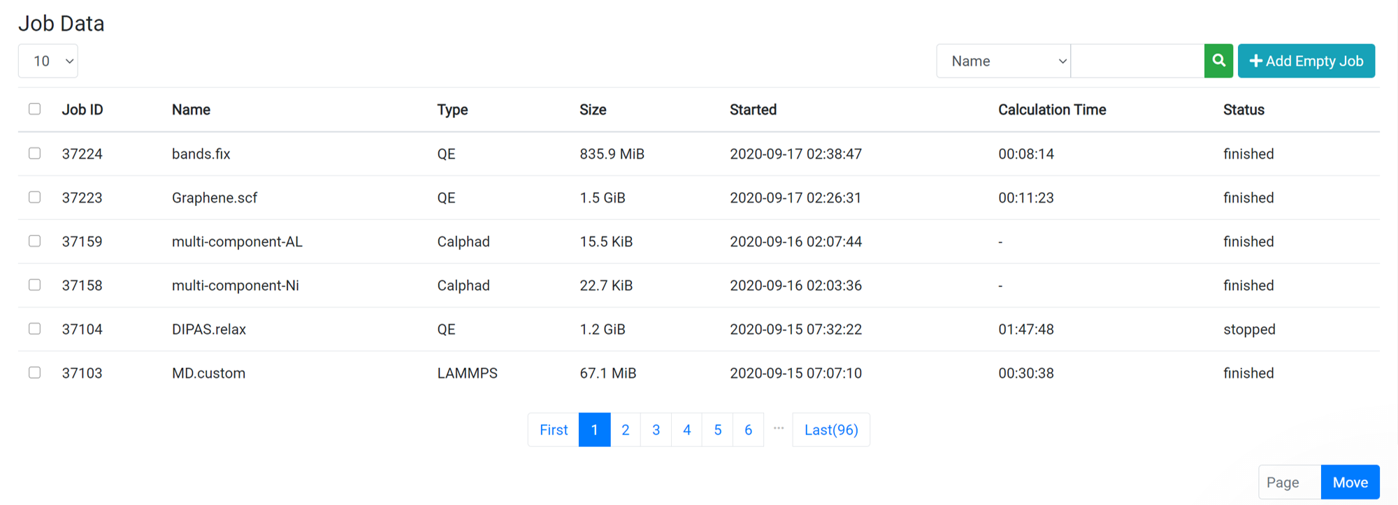
A direct connection to the 'Data' page is enabled from the status bar of the 'Simulation' module. The numbers shown in the parentheses is the job id, which is the unique ID of a job, and you can click on a job id to see its raw data of the calculation.
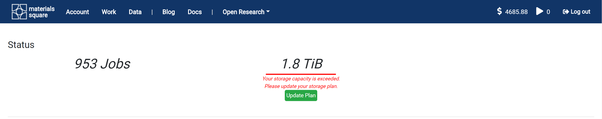
It shows the total number of jobs performed so far and the occupied storage capacity. The default storage capacity is 100 GB. If you need it, you can store more data in the cloud by purchasing a storage plan.
The output of a simulated computation is in the text form by default. If the module does not load the desired data, you can locate the desired data by reading the original data.
 When you click on one of the jobs from the job list on the Data page, the raw data file list is displayed at the same time the Parent Work information is displayed. For information about the files that appear, see the following
File Types and Description:
When you click on one of the jobs from the job list on the Data page, the raw data file list is displayed at the same time the Parent Work information is displayed. For information about the files that appear, see the following
File Types and Description:
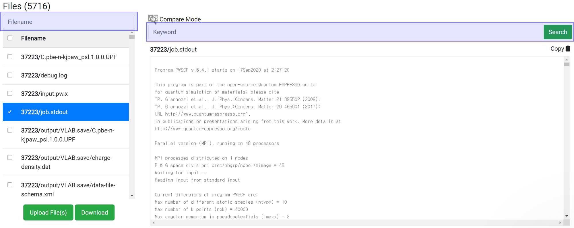
Search enables to show only the desired files or information. This search box does the same function as the 'grep' command in Linux. This search box is case sensitive.
The most important file to check is job.stdout. Most of the output information calculated by Quantum Espresso is written to job.stdout. Therefore, checking this file can yield a lot of data, such as checking energy in the middle of a calculation, verifying convergence, estimating the estimated calculation time, and more.
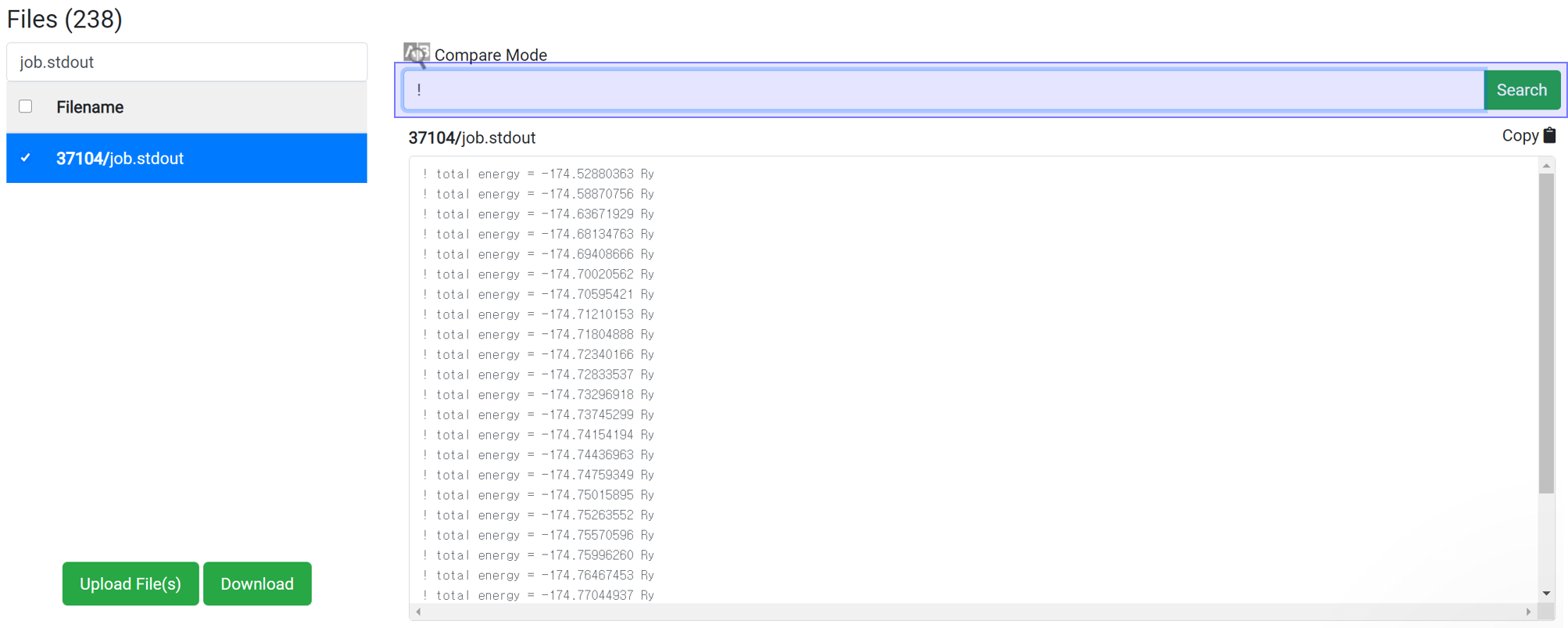 Enter ‘!’ in the Find string search box.
In the PWscf calculation, the one 'total energy' value is created when one SCF algorithm finished. So for SCF calculation, this data can be checked after the calculation ends.
This method can apply for the job with at least 1 iteration finished. Enter 'time' in the Find String search box to display the accumulated calculation time. This information is written at the end of one iteration, and the time takes for each iteration is about the same. So you can use it to estimate the total time.
If the time interval is 30 second and 'Max scf steps' is set to 200 and 'Max iteration steps' is set to 100, the maximum consumption time can be estimated to be 30 * 200 * 100 = 600,000 seconds. In most cases, calculations achieve convergence before reach the max steps of course. This is the maximum time just for the case if the calculation does not achieve convergence until the end.

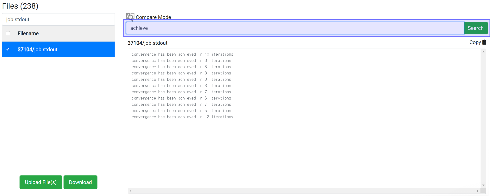
Whether the structure can achieve convergence easily can be estimated by searching for 'achieve'. By typing 'achieve' in the search box, you can see how many iterations took to converge at each scf step. Convergence for highly symmetrical structures takes place in about 10 iterations. If convergence does not occur within the set maximum iteration step, increase the maximum iteration step value or change the accuracy of the initial structure or calculation.
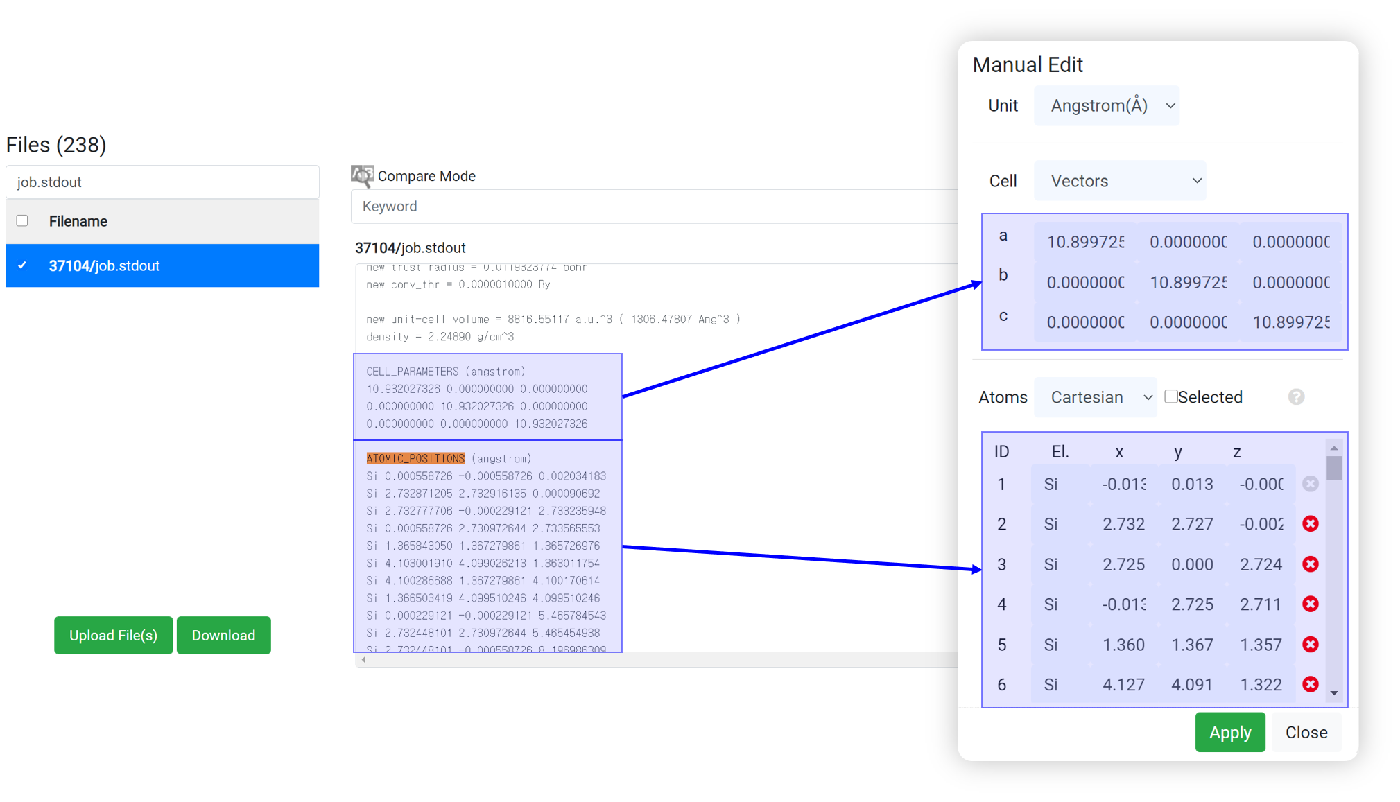
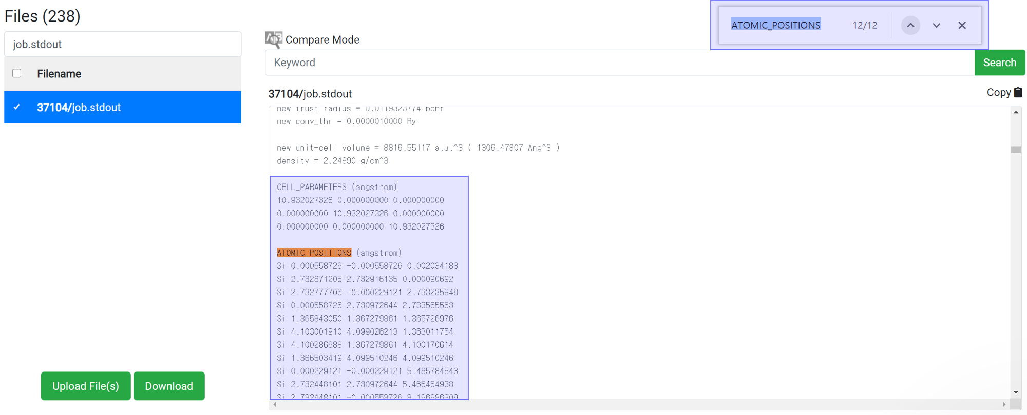 Generally, variable cell relaxation calculation takes many calculation time. To check the structure data in the middle of calculation, find the information at the job.stdout.
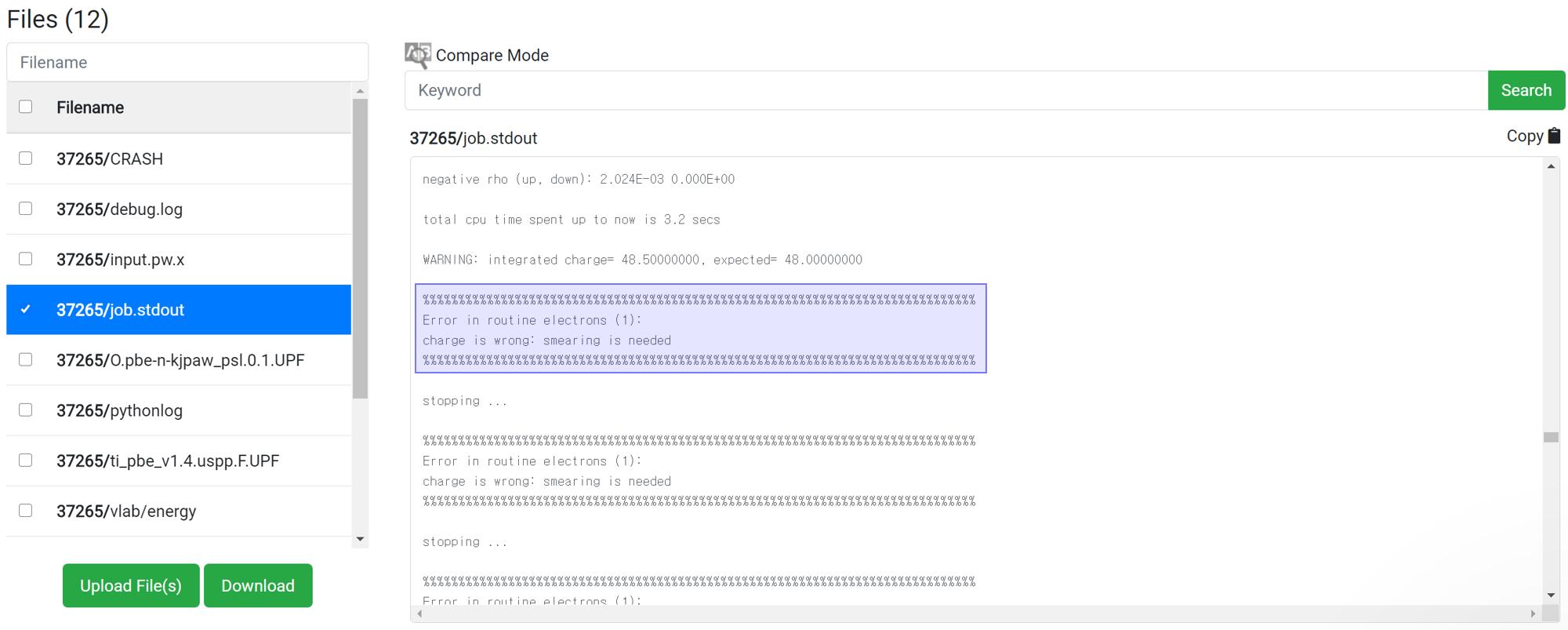
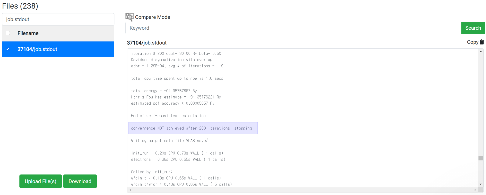
Even if 'This has been finished normally' message is displayed in the module, the calculation may not actually have finished normally. Therefore, before checking the result data, check if the following message is at the bottom of 'job.stdout'.
 For the reason of this error, please refer to
Troubleshooting
.
For the reason of this error, please refer to
Troubleshooting
.
 For the reason of this error, please refer to
Restart
.
For the reason of this error, please refer to
Restart
.
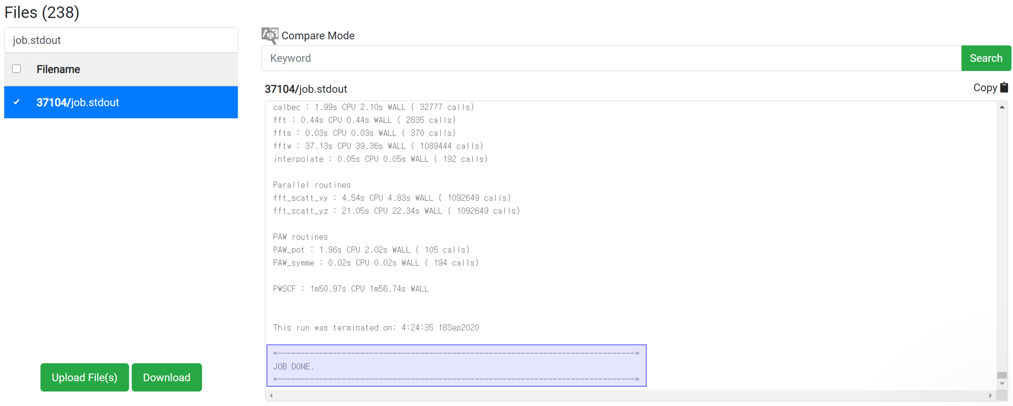 If there is no message like ‘Crash’ or ‘Not Achieved’ as above, the job has ended normally.
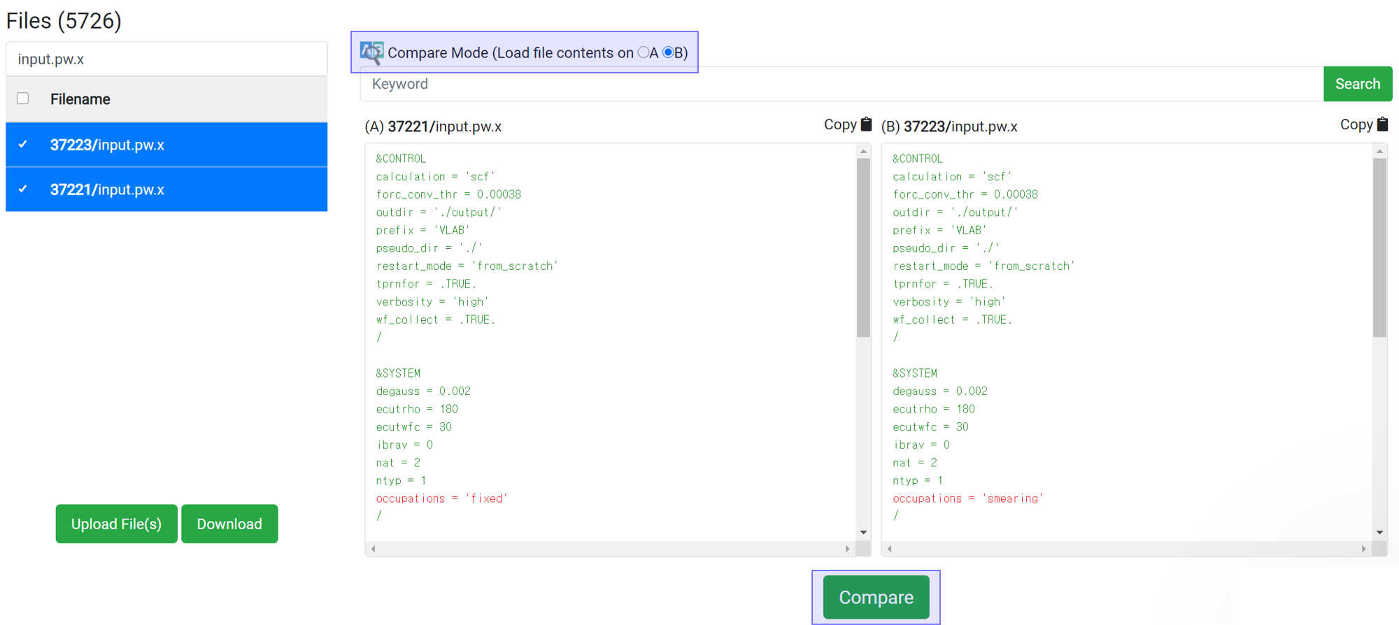 If you want to compare two files, press the
 button to assign the data to A and B. You can compare the files from different jobs by selecting two jobs in the upside 'Job Data' table. The difference between the two files is displayed in the red-colored text after clicking
button.
button to assign the data to A and B. You can compare the files from different jobs by selecting two jobs in the upside 'Job Data' table. The difference between the two files is displayed in the red-colored text after clicking
button.
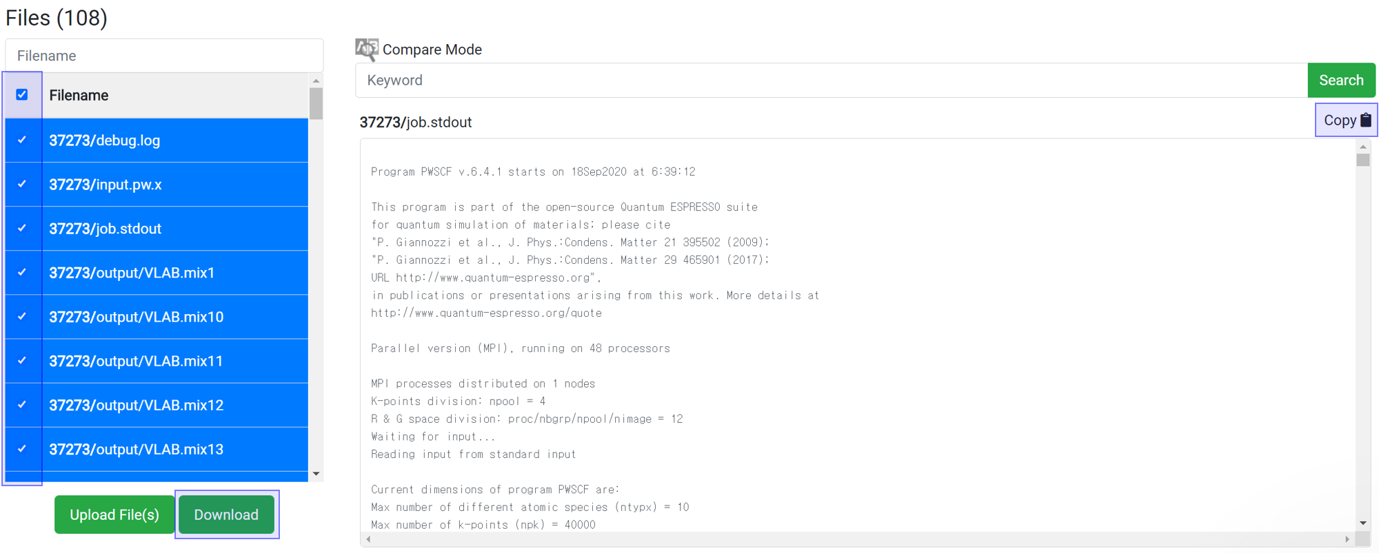 You can download data for further processing of the data. Select the desired files and click the
button to download the selected file only. Alternatively, you can copy and paste all of the text from the contents window into another program from the 'Copy
' button.
You can download data for further processing of the data. Select the desired files and click the
button to download the selected file only. Alternatively, you can copy and paste all of the text from the contents window into another program from the 'Copy
' button.
A direct connection to the 'Data' page is enabled from the status bar of the 'Simulation' module. The numbers shown in the parentheses is the job id, which is the unique ID of a job, and you can click on a job id to see its raw data of the calculation.
It shows the total number of jobs performed so far and the occupied storage capacity. The default storage capacity is 100 GB. If you need it, you can store more data in the cloud by purchasing a storage plan.
The output of a simulated computation is in the text form by default. If the module does not load the desired data, you can locate the desired data by reading the original data.
Search enables to show only the desired files or information. This search box does the same function as the 'grep' command in Linux. This search box is case sensitive.
| File Location | File Name | Description |
|---|---|---|
| input.pw.x | The input script of a PWscf (pw.x) calculation. | |
| job.stdout | The output file of a PWscf (pw.x) calculation containing all data related to the basic calculation. | |
| job.stdout.pp.x | The output file of a Charge Density (pp.x) calculation. | |
| job.stdout.projwfc.x | The output file of a DOS (projwfc.x) calculation. | |
| job.stdout.bands.x | The output file of a Band Structure (bands.x) output calculation. | |
| *.UPF | The pseudopotential file used in calculations. | |
| output/ | VLAB.xml | The file containing the same data as job.stdout. |
| output/ | VLAB.wfc* | The files contain the wavefunction data. It is a large file and is in an unreadable binary format. |
| output/VLAB.save/ | charge-density.dat | The file containing the charge density. |
| output/VLAB.save/ | data-file-schema.xml | The file containing the same data as job.stdout. |
| output/VLAB.save/ | paw.txt | The file created for PAW pseudopotential. |
| output/VLAB.save/ | wfc*.dat | The files contain the wavefunction data. It is a large file and is in an unreadable binary format. |
| vlab/trajectory/ | *.dat | When you perform calculations with multiple scf steps or molecular dynamics calculations, this file saves the movement of the each atom for the snap shots in the trajectory. |
| vlab/trajectory/ | msd | The file containing the msd data. |
| pp.x/ | input.pp.x | The input script file of charge density (pp.x) calculations. |
| pp.x/ | ppoutput.* | The output script file of charge density (pp.x) calculations. |
| pp.x/ | *.cube | The file containing the results corresponding to the plot number selected in charge density (pp.x) calculations. |
| pp.x/ | ACF.dat | It contains atom order number, the coordinates of each atom, the charge associated with it according to Bader partitioning, percentage of the whole according to Bader partitioning and the minimum distance to the surface. |
| pp.x/ | AVF.dat | The number of each volume that has been assigned to each atom. |
| pp.x/ | BCF.dat | It contains the coordinates of each Bader maxima, the charge within that volume, the nearest atom and the distance to that atom. |
| pp.x/ | avg.dat | The output file of the Macroscopic average. The 1, 2, 3 are the results that correspond to the x, y, z-axis. |
| pp.x/ | input.pp.x.avg.in | The input file for the Macroscopic average calcluation. |
| pp.x/ | ppoutput.bader.* | The output file of Bader charge calculation using the charge density. |
| bands.x/ | input.bands.x | The input script file of band structure (bands.x) calculations. |
| bands.x/ | bandsx | The file containing information on each band. |
| bands.x/ | bandsx.gnu | A gnu file for drawing a band structure graph. |
The most important file to check is job.stdout. Most of the output information calculated by Quantum Espresso is written to job.stdout. Therefore, checking this file can yield a lot of data, such as checking energy in the middle of a calculation, verifying convergence, estimating the estimated calculation time, and more.
In the PWscf calculation, the one 'total energy' value is created when one SCF algorithm finished. So for SCF calculation, this data can be checked after the calculation ends.
This method can apply for the job with at least 1 iteration finished. Enter 'time' in the Find String search box to display the accumulated calculation time. This information is written at the end of one iteration, and the time takes for each iteration is about the same. So you can use it to estimate the total time.
If the time interval is 30 second and 'Max scf steps' is set to 200 and 'Max iteration steps' is set to 100, the maximum consumption time can be estimated to be 30 * 200 * 100 = 600,000 seconds. In most cases, calculations achieve convergence before reach the max steps of course. This is the maximum time just for the case if the calculation does not achieve convergence until the end.
Whether the structure can achieve convergence easily can be estimated by searching for 'achieve'. By typing 'achieve' in the search box, you can see how many iterations took to converge at each scf step. Convergence for highly symmetrical structures takes place in about 10 iterations. If convergence does not occur within the set maximum iteration step, increase the maximum iteration step value or change the accuracy of the initial structure or calculation.
- Search ‘ATOMIC_’ text at the search box in the browser (ctrl+F).
- Copy the cell parameter and atomic position information.
- And paste that to the ‘EDIT’ menu in the structure builder module.
Even if 'This has been finished normally' message is displayed in the module, the calculation may not actually have finished normally. Therefore, before checking the result data, check if the following message is at the bottom of 'job.stdout'.
| Template | File name | Description |
|---|---|---|
| Common | job.stdout | The output file of a LAMMPS calculation containing all data related to the LAMMPS calculation. |
| Common | log.lammps | The output file of a LAMMPS calculation containing all data related to the LAMMPS calculation. |
| Common | input.lammps | The input script of LAMMPS calculation. |
| Common | structure.matsq.lammps | The initial structure data of the LAMMPS calculation. |
| Common | #.dat | The trajectory file during LAMMPS calculation. The 'Movie' module only works when the trajectory saved in this format. |
| Calculation Type | File Location | File name | Description |
|---|---|---|---|
| Common | EXTBAS | Generated basis set file when using custom basis set (external basis set) such as LANL2DZ, def2svp | |
| Common | gamess.x.dat | Orbital, Energies, Vibrational modes information file | |
| Common | gamess.x.inp | GAMESS Input file. It contains structural information and designated input parameters | |
| Common | job.stdout | GAMESS Output file. It contains most of the simulation information, such as energy data. | |
| Common | pythonlog | File for data parsing | |
| Common | vlab/ | dos | DOS Spectrum and MO Eigenvalues |
| Common | vlab/ | energy | File for data parsing |
| Common | vlab/ | jsondata | File for data parsing |
| Common | vlab/ | metadata | File for data parsing |
| Common | vlab/ | moenergies | File for data parsing |
| Common | vlab/ | order | File for data parsing |
| Common | vlab/ | status | File for data parsing |
| Common | vlab/ | thermo | File for data parsing |
| Common | vlab/ | valence | File for data parsing |
| Common | vlab/trajectory | #.xyz | Trajectory file generated from geometry optimization |
| NEB | gamess.x.trj | Trajectory file generated from NEB calculation result | |
| NEB | vlab/ | neb_data.json | File for data parsing |
| Hessian | gamess.x.rst | This file need for restart Energy/Gradient/Dipole calculation. It generated when hessian calculation. | |
| BDE | vlab/ | bde_data.json | File for data parsing |